Decision tree and variables having lots of levels

Once a friend of mine asked me what to do with his dataset. He was trying to fit a tree model to the data at hand, but one of the categorical has too many levels. As a result, he felt it was necessary to do “pre-processing” on that variable. This is a common belief among data scientists: categorical variables having too many levels can cause trouble for tree-based models. Documentation of scikit-learn even has a dedicated article on this topic, see [1].

But how many level is too many? Why does large cardinality cause trouble? Does large cardinality always cause trouble? These questions caught my interest and hence we have this blog post now.

It’s not about how many levels $X$ have, but about…?

Data scientists tend to say things like “Oh, my variable $X_2$ has too many levels, so…”. But in reality, it’s not about how many levels $X_2$ have, but about how many partitions it can induce on $Y$. Recall that when a tree makes a split, it will

1. Scan through all the variables $X_1, X_2, \cdots, X_p$
2. For each variable, scan through all the possible partitions on $y_i$’s by which this variable can create. Specifically,
   1. If $X_j$ is numerical and has values $x_{j1},x_{j2},\cdots,x_{jm}$ present in the data, we look at all sets ${y_i \mid x_i \le x_{ik}}$
   2. If $X_j$ is categorical and has levels $a, b, c$ present in the data, then we look at all sets ${y_i \mid x_i \in \text{some subset of } \{a,b,c\}}$
3. Find the best variable and its best split

So, in fact, it’s not that the cardinality of $X_i$ that matters. Rather, it’s the cardinality of the set of partitions it can induce matters. Specifically, if $X_j$ is a categorical variable with $q$ levels, then it creates $2^q - 1$ partitions. On the other hand, if $X_j$ is a numeric with $q$ distinct values, then it creates only $q$ partitions. In fact, that’s why randomForest package in R cannot handle categorical variables with more than 32 categories. Because a categorical variable with 32 cateogires induces 2,147,483,647 partitions on $y_i$’s. See [2].

Sure. But still, if $X$ has many levels, it induces more partitions on $y_i$’s, so it’s always a problem…?

The answer is “yes” most of the time in practice. However, in some sense, the reason lies not in $X$ but other independent variables.

Let us consider a simple example. We simulate $n$ data points from $Y = 3X_1 + \epsilon$ where $\epsilon$ is some noise. Now, we add a categorical variable $X_2$ with many levels. Given the data, will the tree split using $X_1$ or $X_2$?

It is easier to consider two extreme cases. First, let us assume that there is no noise term. That is, $Y = 3X_1$ exactly. In this case, the tree will split using $X_1$ all the time. Even if we have $n$ levels in $X_2$, we will get a tie. On the other hand, if we have $n$ levels in $X_2$ and we have even a little bit noise, the tree always favor $X_2$. This is because any partition induced by $X_1$ can be induced by $X_2$, but not the other way around.

> set.seed(45)
> par(mfrow = c(2, 1))
> x1 <- rnorm(mean = 1, n=100)
> y <- 3*x1
> x2 <- as.factor(seq(1, 100))
> df <- data.frame(x1, x2 = sample(rep_len(x2, length.out = 100)), y)
> 
> fitted_cart <- rpart(y ~ x1 + x2, data=df, method = "anova",
+                      control = rpart.control(minsplit = 2, maxdepth = 1))
> rpart.plot(fitted_cart, main = "Case 1: 100 levels with no noise. Tie.")
> print(fitted_cart$splits)
   count ncat   improve    index adj
x1   100   -1 0.5994785 1.552605   0
x2   100  100 0.5994785 1.000000   0
> 
> 
> # Number of level equals to sample size, with a little bit of noise
> x1 <- rnorm(mean = 1, n=100)
> y <- 3*x1 + rnorm(n = 100, sd = 0.5)
> x2 <- as.factor(seq(1, 100))
> df <- data.frame(x2 = sample(rep_len(x2, length.out = 100)), x1, y)
> 
> fitted_cart <- rpart(y ~ x2 + x1, data=df, method = "anova",
+                      control = rpart.control(minsplit = 2, maxdepth = 1))
> rpart.plot(fitted_cart, main = "Case 2: 100 levels with very little noise")
> print(fitted_cart$splits)
   count ncat   improve     index       adj
x2   100  100 0.6414503 1.0000000 0.0000000
x1   100   -1 0.6371685 0.9917295 0.0000000
x1     0   -1 0.9800000 0.9079153 0.9565217

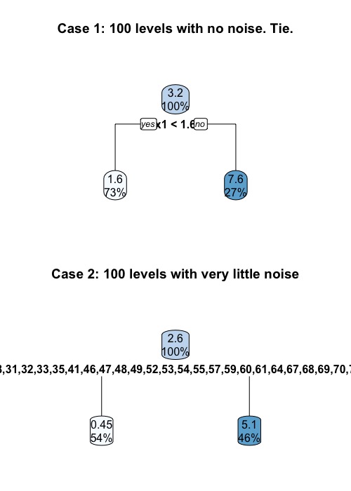
However, as expected, it is more difficult to draw conclusion on any less extreme cases (e.g. We have 1000 data points, and $X_2$ has 20 levels). “How many level is too many?” is a difficult question to answer. However, we can do a simple simulation to get some general idea:

set.seed(42)

library(rpart)

result <- c()
std_list <- seq(0.1, 4, 0.05)
for (std in std_list) {
  fv <- 0
  
  for (cnt in seq(1, 200)) {  # For each std, simulation 200 times
    x1 <- rnorm(mean = 1, n=100)
    y <- 3*x1 + rnorm(n = 100, sd = std)
    x2 <- as.factor(seq(1, 90))
    df <- data.frame(x2 = sample(rep_len(x2, length.out = 100)), x1, y)
    
    fitted_cart <- rpart(y ~ x2 + x1, data=df, method = "anova",
                 control = rpart.control(minsplit = 2, maxdepth = 1))
    
    if (data.frame(rpart.rules(fitted_cart))$Var.3[1] == "x2") {
      fv <- fv + 1
    }
  }
  
  result <- c(result, fv/200)
}

plot(std_list, result,
     xlab = "Standard deviation of noise",
     ylab = "Prob. of choosing the categorical variable X2",
     main = "How often does the tree choose the categorical variable X2?")

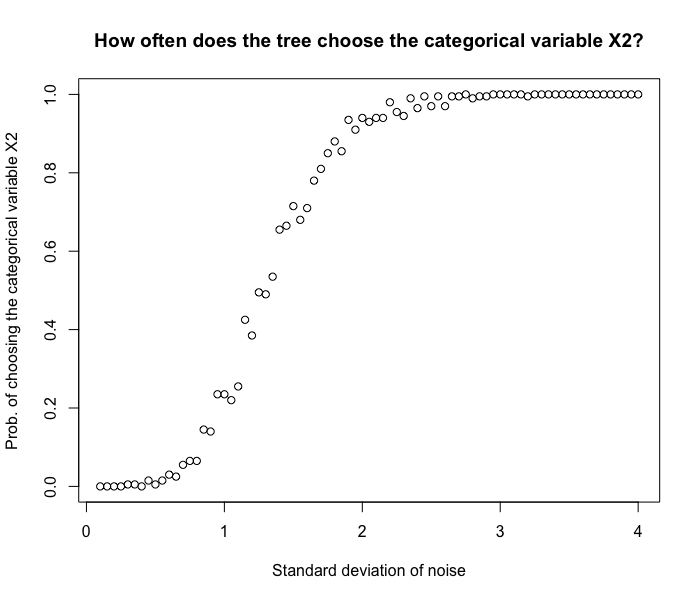
In this simulation, we generate 100 data points. from $Y = 3X_1 + \epsilon$ with different noise levels. We then see how likely the tree will make a split using $X_2$, the unrelated categorical variable with 90 levels. From the graph, we see that

1. Even though we have a cat variable with lots of levels, when the noise level is small, the tree still chooses the right variable $X_1$ to make a split.
2. When the noise level increases, it becomes more and more difficult to make a good split using $X_1$. Since $X_2$ has many levels and creates more partitions on $y_i$’s, the tree tends to use $X_2$.

In order to better understand the role of “noise level/variance level”, we should realize that decision tree has a very interesting property: Even though the whole tree forces all variables to interact with each other, it essentially does a sequence of univariate analysis at each node.

For example, at any given node, it might be the case that two variables gender and year_of_education combined can explain $y_i$’s pretty well, thus reducing the variance. But when we look at them individually, none of them is highly correlated with $y_i$’s. Under such situation, a third unrelated categorical variable with lots of level might be favored. This type of situation is probably very common in practice. So it is very understandable that people think categorical variables with many levels tend to cause problems.

Sample size also matters

It can also be demonstrated that if we keep the number of levels of $X_2$ fixed but increase the sample size, the decision tree becomes less likely to be tricked by $X_2$. This should not be surprising.

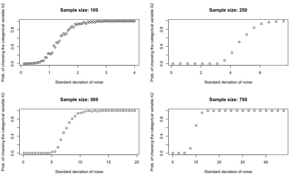
In practice, even though we have a large data set, we might still run into trouble. Because as the tree grows deeper, the sample size within each partition becomes smallers and smaller. For example, if we start with 100,000 data points and we grow our tree 3 levels deep perfectly balanced, we end up with only 12,500 data points.

References:

1. https://scikit-learn.org/stable/auto_examples/inspection/plot_permutation_importance.html#sphx-glr-auto-examples-inspection-plot-permutation-importance-py
2. https://stats.stackexchange.com/questions/49243/rs-randomforest-can-not-handle-more-than-32-levels-what-is-workaround

When we forget to use zero-truncated Poisson model

Poisson model (e.g. Poisson GLM) is often used to model count data. For example, the number of train arrivals for a given time period can be Poisson distributed. This is closely related to Poisson process.

A Poisson variable $X$ can take values in ${0, 1, 2, \cdots}$. However, sometimes the zero’s are censored. For example, the number of car accidents might be Poisson distributed. But, if a vehicle had zero accident, it might not get reported in the first place. We can only observe the non-zero outcomes. In such cases, Poisson is not the appropriate distribution to use. Instead, we should use zero-truncated Poisson distribution. As we will see later, misspecification will lead to incorrect parameter estimates, especially when it is very likely to observe zero.

Probability mass function

Recall that if $X$ is Poisson distributed with mean $\lambda$, then

A truncated Poisson random variable $Z$ has probability mass function

We can show that $\mathbb{E}[Z] = \frac{\lambda}{1 - e^{-\lambda}}$.

MLE based on i.i.d. sample

Assume we have observed $z_1, \cdots, z_n$ from a truncated Poisson distribution with $\lambda$ (that is, the underlying untruncated variable has mean $\lambda$). The correct way to set up MLE estimator is to solve

for $\lambda$, which we denote as $\hat{\lambda}_{MLE, trunc}$.

This has no closed form solution. And this is different from the MLE for the untruncated Poisson, which is just $\hat{\lambda}_{MLE} =\bar{z}_n$. However, if the zero has a fairly small probability (i.e. $e^{-\lambda}$ is very small), then $\hat{\lambda}_{MLE}$ and $\hat{\lambda}_{MLE, trunc}$ will be quite close. This makes intuitive sense.

library(countreg)
library(gridExtra)
library(extraDistr)

sample_size <- seq(10, 5000, 99)
set.seed(233)
# Simple MLE ----
simulate <- function(n = sample_size, lambda = lambda) {
  MLE_trunc <- c()
  MLE <- c()
  
  for (n in sample_size) {
    X_pois <- data.frame(y = rpois(n = n, lambda = lambda))
    X_tpois <- data.frame(y = rtpois(n = n, lambda = lambda, a = 0, b = Inf))
    
    MLE_trunc <- c(MLE_trunc, glm(y ~ ., data = X_tpois, family = ztpoisson)$coefficients %>% exp())
    MLE <- c(MLE, glm(y ~ ., data = X_tpois, family = poisson())$coefficients %>% exp())
  }
  
  plot_df <- data.frame(MLE_trunc, MLE, sample_size) %>%
    tidyr::pivot_longer(cols = c("MLE_trunc", "MLE"))
  
  plot <- ggplot(data = plot_df, aes(x = sample_size, y = value, color = name)) +
    geom_point() +
    geom_hline(yintercept = lambda) +
    labs(title = paste("Lambda: ", lambda)) + xlab("Sample Size") + ylab("Value") +
    theme_minimal()
  return(plot)
}

plot_1 <- simulate(sample_size, lambda = 1)
plot_2 <- simulate(sample_size, lambda = 4)

grid.arrange(plot_1, plot_2, ncol = 1)

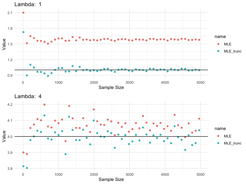
In this simulation, we generate a series of samples from zero-truncated Poisson with $\lambda$ equal to $1$ and $4$, respectively. The blue points are MLE’s estimated based on the correct truncated Poisson likelihood. The red points are MLE’s estimated based on Poisson likelihood, which is incorrect, since the data are not Poisson, but zero-truncated Poisson. We see that

1. $\hat{\lambda}_{MLE,trunc}$ estimates true $\lambda$ consistently
2. $\hat{\lambda}_{MLE}$ does not correctly estimates $\lambda$. However, the bigger the $\lambda$, the smaller the error.

MLE of generalized linear model

Similar conclusion holds for Poisson/zero-truncated Poisson GLM. Under a zero-truncated Poisson GLM (with log-link), observations $y_i$’s are generated form a zero-truncated Poisson distribution:

where $\log(\lambda_i) = x_i^T \beta$.

We first generate 5,000 $(x_1, \cdots, x_5)_i$ from a normal distribution with mean $m$ and s.d. $1$. Then, we generate 5,000 $y_i$ from a zero-truncated Poisson with mean $\lambda := \exp(x_i^T \beta)$, where $\beta = (-0.05, 0.15, -0.25, 0.2, 1)$. The whole process is repeated for different values of $m$’s.

For each $m$, we fit a zero-truncated Poisson GLM and a Poisson GLM. We then compute the MSE between estimates and true parameters.

set.seed(233)
true_param <- c(-0.05, 0.15, -0.25, 0.2, 1)

mse_poisson <- c()
mse_ztpoisson <- c()

for (m in seq(-2, 2, by = 0.025)) {
  X <- matrix(rnorm(n = 5000*5, mean = m, sd = 1), nrow = 5000, ncol = 5) %>% data.frame()
  X$lambda <- exp(-0.05*(X$X1) + 0.15*(X$X2) - 0.25*(X$X3) + 0.2*(X$X4) + 1*(X$X5))
  X$y <- rtpois(n = length(X$lambda), lambda = X$lambda, a = 0, b = Inf)
  X$lambda <- NULL
  
  mse_poisson <- c(mse_poisson, mean((glm2(y ~ . - 1, data = X, family = poisson(), control = list(maxit = 200))$coefficients - true_param)^2))
  mse_ztpoisson <- c(mse_ztpoisson, mean((glm2(y ~ . - 1, data = X, family = ztpoisson(), control = list(maxit = 200))$coefficients - true_param)^2))
}

plot_df <- data.frame(mse_poisson, mse_ztpoisson, lambda = exp(seq(-2, 2, by = 0.025) * sum(true_param))) %>%
  tidyr::pivot_longer(cols = c("mse_poisson", "mse_ztpoisson")) %>%
  arrange(lambda)

ggplot(data = plot_df, aes(x = lambda, y = value, colour = name)) + geom_point() +
  labs(title = "Deviation from true coefficients (MSE)") + xlab("Lambda") + ylab("MSE") +
  theme_minimal()

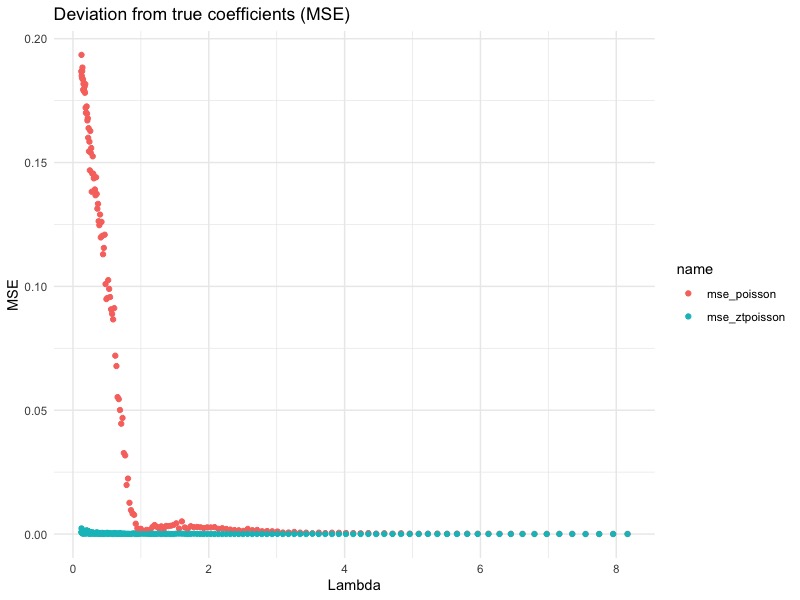
From this plot, we see that the bigger the $\lambda$, the smaller the difference. This agrees with our previous conclusion: When $\lambda$ is large enough, the difference between zero-truncated Poisson and Poisson becomes very small, since $\mathbb{P}[Y_i = 0] = e^{-\lambda} = e^{-e^{x’\beta}}$ becomes negligible. In fact, for this particular simulation, we can see that the difference becomes small when $\lambda = 1$. This translates to $\mathbb{P}[Y_i = 0] = 0.3679$ (abusing notation here). In other words, if the underlying uncensored Poisson variable is zero about 36.79% of the time (or more), than it would be really bad if we forgot to use zero-truncated Poisson GLM.

A popular way of choosing base level in regression revisited (cont'd)

General case: with other covariates

To recap, we want to examine the following statement about choosing base level for a regression model:

Always choose the level with most observations as the reference level, because this gives us a coefficient estimate with smaller variance.

We have shown that this is true for simple regression model. Now we look at multiple regression model.

In general, we have a dummy variable as well as other covariates. Let $\mathbf{X}_{n\times(p+1)}$ be our design matrix where the dummy variable is the last column and the intercept is the first column. For example, our model might be $y_i = \beta_0 + \beta_1 \cdot \text{family_size} + \beta_2 \cdot \text{sex} + \epsilon_i$. Then

represents the same design matrix using different sex as its base level.

We want to show a similar result, that is

1. The variance of $\hat{\beta}_p$ (coefficient corresponds to the dummy variable) does not depend on the choice of reference level.
2. The variance of $\hat{\beta}_0$ depends on the choice of reference level, and we should choose the group with more observations (spoiler alert: this is not true).

How do we find the variance of $\hat{\beta}_p$ ?

We know that $\hat{\beta} = \left(\mathbf{X}’\mathbf{X}\right)^{-1} \mathbf{X}’ \mathbf{y}$ under one representation, and $\hat{\beta} = \left(\mathbf{Z}’\mathbf{Z}\right)^{-1}\mathbf{Z}’ \mathbf{y}$. These two expressions do not help us much. We also know that the variance of $\hat{\beta}_i$ is $\left(\mathbf{X}’\mathbf{X}\right)^{-1}_{ii} \sigma^2$. But finding an explicit expression for $\left(\mathbf{X}’\mathbf{X}\right)^{-1}$ can be difficult, and the algebra can get pretty involved.

Instead, we introduce another identity from [1] and use a geometric argument. Let $V_{p-1}$ be the vector space spanned by column $\mathbf{x}_1$ (the intercept), $\mathbf{x}_2, \cdots, \mathbf{x}_{p-1}$. We can project $\mathbf{x}_p$ onto $V_{p-1}$, and we denote the projected vector as $p\left(\mathbf{x}_p \mid V_{p-1}\right)$. Equivalently, we can write $\mathbf{P} \mathbf{x}_p$ where $\mathbf{P}$ is the corresponding projection matrix.

Then, we define $ \mathbf{x}_p^\perp = \mathbf{x}_p - p(\mathbf{x}_p \mid V_{p-1}) $. According to [1], we can express the variance as

Now let’s study the variance of $\hat{\beta}_p$ under different base level. This reduces to comparing $|\mathbf{x}_p^\perp|^2$ with $|\mathbf{z}_p^\perp|^2$.

Assume that when we use female as base level, the last column is $\mathbf{x}_p$. Then if we use male as reference level, the last column becomes $\mathbf{z}_p := \mathbf{1} - \mathbf{x}_p$. To compare, we write

We want to show that those two are equal. After some algera, we get

Notice that since $\mathbf{1}$ is in the subspace $V_{p-1}$ (since $V_{p-1}$ contains the first column, which is the intercept), $\mathbf{P} \mathbf{1} = \mathbf{1}$. So the term $\langle \mathbf{P} \mathbf{1} - \mathbf{1}, \mathbf{x} - \mathbf{1}\rangle$ vanishes. Also, since $\mathbf{P}$ is a projection and $\mathbf{1}$ is in the space on which we project, $\mathbf{x}_p - \mathbf{P}\mathbf{x}_p$ is orthogonal to $\mathbf{1}$. So $\langle \mathbf{x}_p - \mathbf{P}\mathbf{x}_p, -\mathbf{1}\rangle$ vanishes, too.

This proves the first statement.

Counterexamples of statement 2

Statement 2 sounds plausible but it is false. To be fair, we have run into multiple cases where using more populous category as base level gives a smaller standard error on the intercept coefficient. However, there are numerous counterexamples. We have found one using the mtcars data that comes with R.

> # vs stands for engine type (0 = V-shaped, 1 = straight).
> # we have 18 V-shapes, and 14 straight
> cars <- mtcars[, c("mpg","cyl","disp","vs")]
> cars$intercept <- rep(1, nrow(cars))
> colnames(cars)[4] <- "vs_straight"
> print(paste("Using group with more obs as reference level?", sum(cars$vs_straight == 1) < sum(cars$vs_straight == 0)))
[1] "Using group with more obs as reference level? TRUE"
> lm(mpg ~ . - 1, data = cars) %>% summary() %>% coef()
              Estimate Std. Error    t value     Pr(>|t|)
cyl         -1.7504373 0.87235809 -2.0065582 5.454156e-02
disp        -0.0202937 0.01045432 -1.9411790 6.236295e-02
vs_straight -0.6337231 1.89593627 -0.3342534 7.406791e-01
intercept   35.8809111 4.47351580  8.0207409 9.819906e-09
> 
> cars$vs_V_shapes <- 1 - cars$vs_straight
> cars$vs_straight <- NULL
> print(paste("Using group with more obs as reference level?", sum(cars$vs_V_shapes == 1) < sum(cars$vs_V_shapes == 0)))
[1] "Using group with more obs as reference level? FALSE"
> lm(mpg ~ . - 1, data = cars) %>% summary() %>% coef()
              Estimate Std. Error    t value     Pr(>|t|)
cyl         -1.7504373 0.87235809 -2.0065582 5.454156e-02
disp        -0.0202937 0.01045432 -1.9411790 6.236295e-02
intercept   35.2471880 3.12535016 11.2778365 6.348795e-12
vs_V_shapes  0.6337231 1.89593627  0.3342534 7.406791e-01

The first regression is run using V-shaped engine (which has more observations) as base level. Yet, the standard error of the intercept is 4.47, much larger than what we get by using straight engine (which has fewer observations) as base level. Also, note that the standard error of vs_straight and vs_V_shapes are the same, as we expect.

In this example, we have 32 observations. They are not equally distributed to two categories (14 obs vs 18 obs), but close. Here is another less balanced example, where we have 20 observations with 15 males. When we use male as base level, the standard error of the intercept coefficient is actually slightly larger.

> set.seed(64)
> n <- 20
> n_m <- 15  # First 15 obs of 20 are males
> 
> dummy_var <- matrix(c(rep(1, n_m), rep(0, n - n_m)), nrow = n)  # Use minority group (female) as base level
> y <- rnorm(20)
> C <- matrix(rpois(n*6, lambda = 6), nrow = n)
> X <- cbind(C, dummy_var, y)
> X <- data.frame(X)
> colnames(X)[7] <- "dummy_var"
> 
> lm(y ~ ., X) %>% summary() %>% coef()
                Estimate Std. Error     t value  Pr(>|t|)
(Intercept)  1.418429502  2.8457756  0.49843337 0.6271886
V1          -0.138312337  0.1547772 -0.89362221 0.3890947
V2           0.161704256  0.1420289  1.13853095 0.2771187
V3           0.011231707  0.1439728  0.07801269 0.9391037
V4          -0.006552859  0.1418405 -0.04619879 0.9639117
V5          -0.329203038  0.1899600 -1.73301198 0.1086883
V6          -0.032312033  0.1480165 -0.21830024 0.8308635
dummy_var    0.256849636  0.6964661  0.36878986 0.7187088
> 
> X$dummy_var <- 1 - X$dummy_var  # Now use majority group (male) as base level
> lm(y ~ ., X) %>% summary() %>% coef()
                Estimate Std. Error     t value  Pr(>|t|)
(Intercept)  1.675279138  2.8950661  0.57866697 0.5735149
V1          -0.138312337  0.1547772 -0.89362221 0.3890947
V2           0.161704256  0.1420289  1.13853095 0.2771187
V3           0.011231707  0.1439728  0.07801269 0.9391037
V4          -0.006552859  0.1418405 -0.04619879 0.9639117
V5          -0.329203038  0.1899600 -1.73301198 0.1086883
V6          -0.032312033  0.1480165 -0.21830024 0.8308635
dummy_var   -0.256849636  0.6964661 -0.36878986 0.7187088

Reference:

1. Linear Statistical Models Second Edition. James H. Stapleton. Wiley. Section 3.5

I appreciate my friend Changyuan Lyu for taking time to discuss this problem with me.

A popular way of choosing base level in regression revisited

First part written on February 13th, 2020.

Set the base level to be one with populous data?

Let’s say you are running a multiple linear regression model, and you have a categorical variable (e.g. sex, which can be male or female). How do you choose the reference level (or base level) for the dummy variable? For example, if you choose “male” as the reference level, then you would define the dummy variable like this:

Interestingly, there is a widely circulated rule on how to choose the reference level:

Always choose the level with the most observations as the base level, because this gives us a coefficient estimate with a smaller variance.

Many people have told me something similar and they work in different industries as statisticians/data scientists. I am not the only one who has experience that, neither. For example, see [1]. There are some resources that approve this approach although they do not present a rigorous study/proof. For example, see [2] and [3].

This is a strong statement, and I will investigate to what extent it is true. To save you some time,

TL;DR:

1. In simple linear regression, this statement is true and can be proved mathematically.
2. In multiple linear regression, this is not always true, as we can find counter-examples easily. But it is 50% true.
3. In GLM, I do not know.

Let’s dive into it.

Simple case: $y_i = \beta_0 + \beta_1 \cdot \text{sex} + \epsilon_i$

Let’s consider a simple case first. We have observations $\left(d_1, y_1\right), \cdots, \left(d_n, y_n\right)$ and commonly-seen assumptions of linear regression are satisfied. The dummy variable is the only covariate, and indicates the sex of each observation. We assume there are only 2 possibilities: male, female. We consider model

Assume there are $n_m$ males, and $n_f$ females. Should we choose male or female as the base level?

We claim that we should choose whichever level that has more observations. Specifically, we will prove 2 statements:

1. Regardless of the reference level, $\text{Var}\left[\hat{\beta}_1\right] = \frac{\sigma^2}{n_m} + \frac{\sigma^2}{n_f}$.
2. If female is the base level (we mark $D_i = 1$ when $i$ is male), then $\text{Var}\left[\hat{\beta}_0\right] = \frac{\sigma^2}{n_f}$. If male is the base level, then $\text{Var}\left[\hat{\beta}_0\right] = \frac{\sigma^2}{n_m}$. So we should choose the female as base level if $n_f \ge n_m$.

One interesting things: the choice of base level has no impact on the variance of $\hat{\beta}_1$, the coefficient estimate of the dummy variable. In other words, choosing the “correct” base level leads to a better model by estimating the intercept better.

Proof of 1: We know that

from which we can derive that

If female is the reference level, then $d_i = 1$ when the $i$-th observation is male. So

if we recall that $n_m + n_f = n$.

Proof of 2: We know that

from which we can derive that

Assume female is the reference level, then $\bar{d}^2 = n_m^2 / n^2$, and $\sum \left(d_i - \bar{d}\right)^2 = n_m n_f/n$. So the variance (omitting $\sigma^2$) becomes

Now assume male is the reference level, then $\bar{d}^2 = n_f^2/n$. Similar derivation shows that statement 2 is true.

To be continued in the next post.

References:

1. https://stats.stackexchange.com/questions/208329/reference-level-in-glm-regression
2. Page 15 of https://www.casact.org/pubs/monographs/papers/05-Goldburd-Khare-Tevet.pdf
3. https://www.theanalysisfactor.com/strategies-dummy-coding/

Some thoughts on "trend" of time series

Everyone agrees that you should care about the “trend” in your time series. For example, it is a common practice to “decompose” your time series into 3 components: trend, seasonality, and randomness. You can do this easily in R using decompose(). However, decomposition might not be as useful as you might think, and sometimes it only confirms your bias.

Data scientists use the term “trend” loosely. Most of the time, when they say “I see an upward trend”, they mean exactly that: The plot goes upward. If a data scientist, with this assumption, use decompose() to decompose the time series at hand, he will only see a smoothed version of the original time series.

As a result, he might be tricked into thinking “there is indeed an upward trend, and statistics (?) just proved it!”. But consider the following two time series:

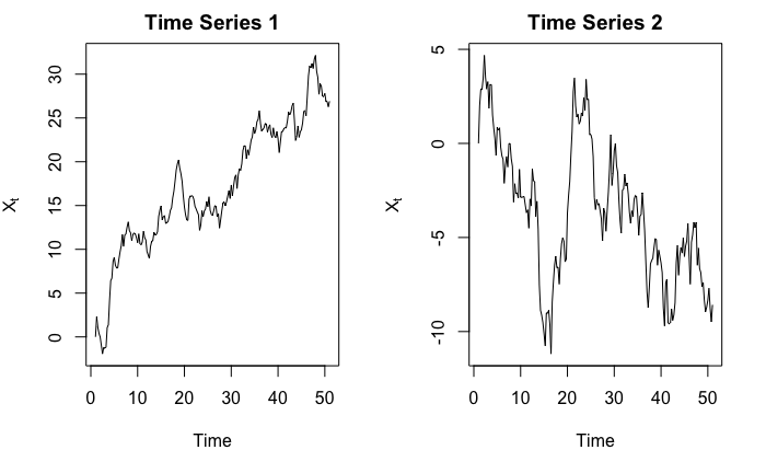
Obviously, in the first graph we see an upward trend, and in the second graph we see a downward trend. Right?

In fact, they are both simulated from $Y_t = Y_{t-1} + \epsilon_t$ where $\epsilon_t \sim N(0,1)$, and $Y_1 = 0$. So $\mathbb{E}\left[X_t\right] = 0$ for all $t$. The observed $X_t$’s indeed go up, but it would be quite ridiculous to say $X_t$ has an upward trend when we, in fact, know that $\mathbb{E}\left[X_t\right] = 0$.

Here is the code used to generate those two series

set.seed(7)

simulate_randomwalk <- function(X_init = 0, noise_mean = 0, noise_var = 1, n_step) {
  ret = c(X_init)
  for (i in 1:n_step) {
    ret <- c(ret, ret[length(ret)] + rnorm(1, noise_mean, noise_var))
  }
  ts(ret)
}

par(mfrow = c(1, 2))
ts_1 <- simulate_randomwalk(n_step = 200) %>% ts(frequency = 4)
plot(ts_1, ylab = expression(X[t]), main = "Time Series 1")

ts_2 <- simulate_randomwalk(n_step = 200) %>% ts(frequency = 4)
plot(ts_2, ylab = expression(X[t]), main = "Time Series 2")

Simply by looking at the shape of the curve does not benefit us much. In practice, we should use context of the data and existing domain knowledge to help us determine if there is any trend or not. In fact, this probably is the only way because we cannot prove there exists a trend mathematically. For example, consider the following example:

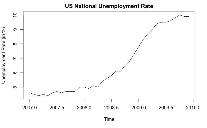
In this example, we can confidently say that an upward trend exists, not because the curve goes up, but because we know what the curve stands for: unemployment rate. From economic theories (or common sense), a 5% increase in unemployment rate cannot possibly be due to “randomness” and is considered to be very significant. Also, if we look at the x-axis, we know that the upward trend is supported by the financial crisis happened around 2008.

To summarize, as Jonathan D. Cryer and Kung-Sik Chan put in their book Time Series Analysis With Applications in R,

“Trends” can be quite elusive. The same time series may be viewed quite differently by different analysts.