When we forget to use zero-truncated Poisson model

Poisson model (e.g. Poisson GLM) is often used to model count data. For example, the number of train arrivals for a given time period can be Poisson distributed. This is closely related to Poisson process.

A Poisson variable $X$ can take values in ${0, 1, 2, \cdots}$. However, sometimes the zero’s are censored. For example, the number of car accidents might be Poisson distributed. But, if a vehicle had zero accident, it might not get reported in the first place. We can only observe the non-zero outcomes. In such cases, Poisson is not the appropriate distribution to use. Instead, we should use zero-truncated Poisson distribution. As we will see later, misspecification will lead to incorrect parameter estimates, especially when it is very likely to observe zero.

Probability mass function

Recall that if $X$ is Poisson distributed with mean $\lambda$, then

A truncated Poisson random variable $Z$ has probability mass function

We can show that $\mathbb{E}[Z] = \frac{\lambda}{1 - e^{-\lambda}}$.

MLE based on i.i.d. sample

Assume we have observed $z_1, \cdots, z_n$ from a truncated Poisson distribution with $\lambda$ (that is, the underlying untruncated variable has mean $\lambda$). The correct way to set up MLE estimator is to solve

for $\lambda$, which we denote as $\hat{\lambda}_{MLE, trunc}$.

This has no closed form solution. And this is different from the MLE for the untruncated Poisson, which is just $\hat{\lambda}_{MLE} =\bar{z}_n$. However, if the zero has a fairly small probability (i.e. $e^{-\lambda}$ is very small), then $\hat{\lambda}_{MLE}$ and $\hat{\lambda}_{MLE, trunc}$ will be quite close. This makes intuitive sense.

library(countreg)
library(gridExtra)
library(extraDistr)

sample_size <- seq(10, 5000, 99)
set.seed(233)
# Simple MLE ----
simulate <- function(n = sample_size, lambda = lambda) {
  MLE_trunc <- c()
  MLE <- c()
  
  for (n in sample_size) {
    X_pois <- data.frame(y = rpois(n = n, lambda = lambda))
    X_tpois <- data.frame(y = rtpois(n = n, lambda = lambda, a = 0, b = Inf))
    
    MLE_trunc <- c(MLE_trunc, glm(y ~ ., data = X_tpois, family = ztpoisson)$coefficients %>% exp())
    MLE <- c(MLE, glm(y ~ ., data = X_tpois, family = poisson())$coefficients %>% exp())
  }
  
  plot_df <- data.frame(MLE_trunc, MLE, sample_size) %>%
    tidyr::pivot_longer(cols = c("MLE_trunc", "MLE"))
  
  plot <- ggplot(data = plot_df, aes(x = sample_size, y = value, color = name)) +
    geom_point() +
    geom_hline(yintercept = lambda) +
    labs(title = paste("Lambda: ", lambda)) + xlab("Sample Size") + ylab("Value") +
    theme_minimal()
  return(plot)
}

plot_1 <- simulate(sample_size, lambda = 1)
plot_2 <- simulate(sample_size, lambda = 4)

grid.arrange(plot_1, plot_2, ncol = 1)

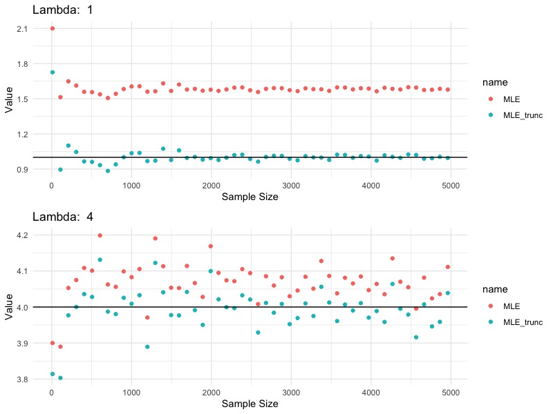
In this simulation, we generate a series of samples from zero-truncated Poisson with $\lambda$ equal to $1$ and $4$, respectively. The blue points are MLE’s estimated based on the correct truncated Poisson likelihood. The red points are MLE’s estimated based on Poisson likelihood, which is incorrect, since the data are not Poisson, but zero-truncated Poisson. We see that

1. $\hat{\lambda}_{MLE,trunc}$ estimates true $\lambda$ consistently
2. $\hat{\lambda}_{MLE}$ does not correctly estimates $\lambda$. However, the bigger the $\lambda$, the smaller the error.

MLE of generalized linear model

Similar conclusion holds for Poisson/zero-truncated Poisson GLM. Under a zero-truncated Poisson GLM (with log-link), observations $y_i$’s are generated form a zero-truncated Poisson distribution:

where $\log(\lambda_i) = x_i^T \beta$.

We first generate 5,000 $(x_1, \cdots, x_5)_i$ from a normal distribution with mean $m$ and s.d. $1$. Then, we generate 5,000 $y_i$ from a zero-truncated Poisson with mean $\lambda := \exp(x_i^T \beta)$, where $\beta = (-0.05, 0.15, -0.25, 0.2, 1)$. The whole process is repeated for different values of $m$’s.

For each $m$, we fit a zero-truncated Poisson GLM and a Poisson GLM. We then compute the MSE between estimates and true parameters.

set.seed(233)
true_param <- c(-0.05, 0.15, -0.25, 0.2, 1)

mse_poisson <- c()
mse_ztpoisson <- c()

for (m in seq(-2, 2, by = 0.025)) {
  X <- matrix(rnorm(n = 5000*5, mean = m, sd = 1), nrow = 5000, ncol = 5) %>% data.frame()
  X$lambda <- exp(-0.05*(X$X1) + 0.15*(X$X2) - 0.25*(X$X3) + 0.2*(X$X4) + 1*(X$X5))
  X$y <- rtpois(n = length(X$lambda), lambda = X$lambda, a = 0, b = Inf)
  X$lambda <- NULL
  
  mse_poisson <- c(mse_poisson, mean((glm2(y ~ . - 1, data = X, family = poisson(), control = list(maxit = 200))$coefficients - true_param)^2))
  mse_ztpoisson <- c(mse_ztpoisson, mean((glm2(y ~ . - 1, data = X, family = ztpoisson(), control = list(maxit = 200))$coefficients - true_param)^2))
}

plot_df <- data.frame(mse_poisson, mse_ztpoisson, lambda = exp(seq(-2, 2, by = 0.025) * sum(true_param))) %>%
  tidyr::pivot_longer(cols = c("mse_poisson", "mse_ztpoisson")) %>%
  arrange(lambda)

ggplot(data = plot_df, aes(x = lambda, y = value, colour = name)) + geom_point() +
  labs(title = "Deviation from true coefficients (MSE)") + xlab("Lambda") + ylab("MSE") +
  theme_minimal()

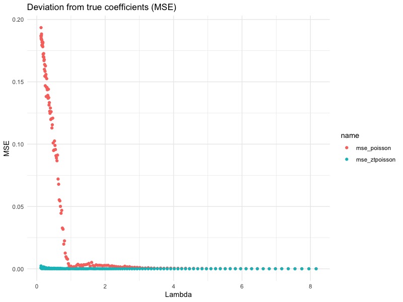
From this plot, we see that the bigger the $\lambda$, the smaller the difference. This agrees with our previous conclusion: When $\lambda$ is large enough, the difference between zero-truncated Poisson and Poisson becomes very small, since $\mathbb{P}[Y_i = 0] = e^{-\lambda} = e^{-e^{x’\beta}}$ becomes negligible. In fact, for this particular simulation, we can see that the difference becomes small when $\lambda = 1$. This translates to $\mathbb{P}[Y_i = 0] = 0.3679$ (abusing notation here). In other words, if the underlying uncensored Poisson variable is zero about 36.79% of the time (or more), than it would be really bad if we forgot to use zero-truncated Poisson GLM.