Logistic regression complete separation - Behind the scene

What is complete separation?

Assume we have data points $(x_i, y_i)$ where $y_i \in {0, 1}$, a binary label. Logistic regression seeks a hyperplane defined by a coefficient vector $\beta$, such that the hyperplane will separate $0$’s and $1$’s nicely. Specifically, if $x_i \beta > 0$, then we predict that $y_i = 1$. Else, then we predict that $y_i = 0$.

Often, it is impossible to correctly classify $0$’s and $1$’s perfectly with a hyperplane, and we will make some mistakes. However, occasionally, we can find a hyperplane that separates them perfectly. This is called complete separation.

Complete separation does not play well with logistic regression. This is a widely known fact to practitioners. When there is complete separation, logistic regression gives extreme coefficient estimate and estimated standard error, which pretty much renders meaningful statistical inference impossible.

A typical R output and its error messages

Typically, this is what you would see in R if there is complete separation. Let’s create some fake data points.

x <- c(-1,-2,-3,1,2,3)
y <- as.factor(c(1,1,1,0,0,0))
df <- data.frame(x, y)
model <- glm(y ~ x + 0, data = df, family = "binomial")

R would give you the following result and warning

Warning message:
glm.fit: fitted probabilities numerically 0 or 1 occurred 

If you choose to ignore the warning and proceed to see the summary anyway,

> summary(model)

Call:
glm(formula = y ~ x + 0, family = "binomial", data = df)

Deviance Residuals: 
         1           2           3           4           5           6  
 1.253e-05   2.110e-08   2.110e-08  -1.253e-05  -2.110e-08  -2.110e-08  

Coefficients:
  Estimate Std. Error z value Pr(>|z|)
x   -23.27   48418.86       0        1

(Dispersion parameter for binomial family taken to be 1)

    Null deviance: 8.3178e+00  on 6  degrees of freedom
Residual deviance: 3.1384e-10  on 5  degrees of freedom
AIC: 2

Number of Fisher Scoring iterations: 24

The first thing that should pop out is the estimated s.e. being 48418.85, which is quite big. A big estimated s.e. leads to a strange looking Z-value and p-value, too.

If you know what “deviance” or “AIC” means, you would notice something else that is strange. For example, we know that $\text{AIC} = -2\ell + 2p$ where $\ell$ is the log-likelihood, and $p$ is the number of parameters. Here, $\text{AIC} = 2$, and we know that $p = 1$. Solving for $\ell$, we get that $\ell = 0$. This means that the likelihood of the model is $1$, which is extremely huge. You can also use logLik(model) to find the log-likelihood of a model object.

> logLik(model)
'log Lik.' -1.569194e-10 (df=1)

Why huge log-likelihood?

Recall that logistic regression is essentially a GLM where $y_i$’s are Bernoulli random variables such that

MLE seeks to maximize

with respect to $\beta$.

Mathematically, if there exists some $\beta$ such that

1. $x_i \beta > 0$ for all $i$ such that $y_i = 1$, and
2. $x_i \beta < 0$ for all $i$ such that $y_i = 0$,

then the hyperplane defined by $\beta$ completely separate $y_i$’s.

A key observation is that if $\beta$ completely separate $y_i$’s, then making $\beta$ arbitrarily larger still completely separates $y_i$’s (since the two inequalities still hold). As a result, if we let $\beta \to \infty$, both terms (which are logarithms of estimated probabilities) in the log-likelihood $\ell$ will go to zero.

This explains why the log-likelihood $\ell$ is close to zero and $\hat{\beta}$ is big as well when there is complete separation, as well as the error message “fitted probabilities numerically 0 or 1 occurred “.

Why huge standard error?

The standard error comes from the Hessian matrix $\mathbf{H}$ of the log-likelihood $\ell$. To be specific, the standard error of $\hat{\beta}_i$ is the $i$-th diagonal entry of $[-\mathbf{H}]^{-1}$. It can be shown that the Hessian matrix of $\ell$ is

where $\hat{p}_i$ is the predicted probability on the $i$-th observation. That is,

Thus, to explain the huge standard error, we can show that

and $\left[-\mathbf{H}\right]_{ii}$ is small when there is complete separation.

If we consider the simple case where we only have 1 covariate, then the estimated standard error is

Due to complete separation, $\hat{p}_i$’s are very close to 1 for each $i$’s, so $\text{s.e.}(\beta)$ will be large, since we are taking reciprocal of something that is close to zero.

In the case where we have $p$ covariates $\beta_1,\cdots,\beta_p$. we need to invert the matrix $-\mathbf{H}$. Consider a SVD written as $\mathbf{P}\mathbf{D}\mathbf{P}^T$ whose inverse is $\mathbf{P} \mathbf{D}^{-1} \mathbf{P}^T$. We need to compare

We have

Using AM-GM inequality, we conclude that

As a result, we have

Since

and this is close to zero when $\hat{p}_i$ is almost 1, we will get a large estimated s.e.

A simple restricted OLS estimator

Last week, I attended a presentation on how to estimate large loss trend. The presentation was interesting, and raised the following question: how to incorporate prior knowledge into estimation, so that the uncertainy of the model can be reduced? This is, of course, a very important and widely-studied question. In fact, one reason why Bayesian statistics attract people is that it can incorporate prior knowledge into the model.

However, since the presentation used a frequentist model, and I am more comfortable with frequentist statistics, I was inspired to think about the following simple question, which is an interesting small exercise:

Question

Consider a simple linear regression model $y_i = \beta_0 + \beta_1 x_i + \epsilon_i$ where the commonly seen assumptions about regression model hold. Here, $\beta_1 > 0$. Denote the OLS estimator of $\beta_1$ as $\hat{\beta}_1$, and define $\hat{\beta}_1^+ = \max \{0, \hat{\beta}_1 \}$. Compare the performance of $\hat{\beta}_1$ and $\hat{\beta}_1^+$.

In other words, since we already know that $\beta_1$ cannot be negative, we will “shrink” the OLS estimator we get $\hat{\beta}_1$ to zero if it is negative.

Unbiasedness

By doing so, obviously we no longer have an unbiased estimator. This is simply because, well, $\hat{\beta}_1$ is unbiased and $\hat{\beta}_1 \ne \hat{\beta}_1^+$. In fact, since $\mathbb{P}\{ \hat{\beta}_1^+ \le t\} = 0$ when $t < 0$, we can actually find an expression for the bias of $\hat{\beta}_1+$.

where $f_{\hat{\beta}_1}$ is the probability density of $\hat{\beta}_1$, the OLS estimator. This has an interesting indication: If $\hat{\beta}_1$ has large variance, than the bias will be large, too. If $\hat{\beta}_1$ has smaller variance, than the bias will not be as big. This makes intuitive sense because if $\hat{\beta}_1$ has smaller variance, than there is a smaller chance for it to be below zero (Remember, we know that $\beta_1 > 0$ and $\hat{\beta}_1$ estimates $\beta_1$ with no bias).

Variance

By sacrificing unbiasedness, hopefully we would get something in return. This is indeed the case since $\hat{\beta}_1^+$ has smaller variance. To prove this, simply notice that

We have \(\text{Var}\left[ \hat{\beta}_1\right] = \text{Var}\left[ \hat{\beta}_1^+\right] + \text{Var}\left[\hat{\beta}_1^-\right] + 2\text{Cov}\left[ \hat{\beta}_1^+, \hat{\beta}_1^-\right]\)

It suffices to prove that the covariance term is non-negative. This is conceivably true, since when $\hat{\beta}_1^+$ goes from zero to some positive number, $\hat{\beta}_1^-$ goes from negative to zero, thus moving in the same direction. Formally,

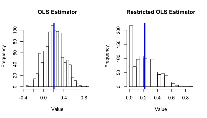
We can also run a small numerical simulation.

set.seed(64)

beta_1_hat_list <- c()
beta_1_hat_c_list <- c()

for (i in 1:1000) {
  beta_0 <- 0.2
  beta_1 <- 0.2
  x <- rnorm(1000, mean = 0.2, sd = 0.8)
  y <- beta_0 + x*beta_1 + rnorm(1000, mean = 1, sd = 5)
  
  beta_1_hat <- sum((x-mean(x))*y) / sum(var(x)*999)
  beta_1_hat_c <- max(beta_1_hat, 0)
  
  beta_1_hat_list <- c(beta_1_hat_list, beta_1_hat)
  beta_1_hat_c_list <- c(beta_1_hat_c_list, beta_1_hat_c)
}

par(mfrow = c(1, 2))
hist(beta_1_hat_list, main = "OLS Estimator", xlab = "Value", breaks = 20)
abline(v = mean(beta_1_hat_list), col = "blue", lwd = 4)
hist(beta_1_hat_c_list, main = "Restricted OLS Estimator", xlab = "Value", breaks = 15)
abline(v = mean(beta_1_hat_c_list), col = "blue", lwd = 4)

The average of 1000 $\hat{\beta}_1^+$ is around 0.220, while the average of $\hat{\beta}_1$ is around 0.207.

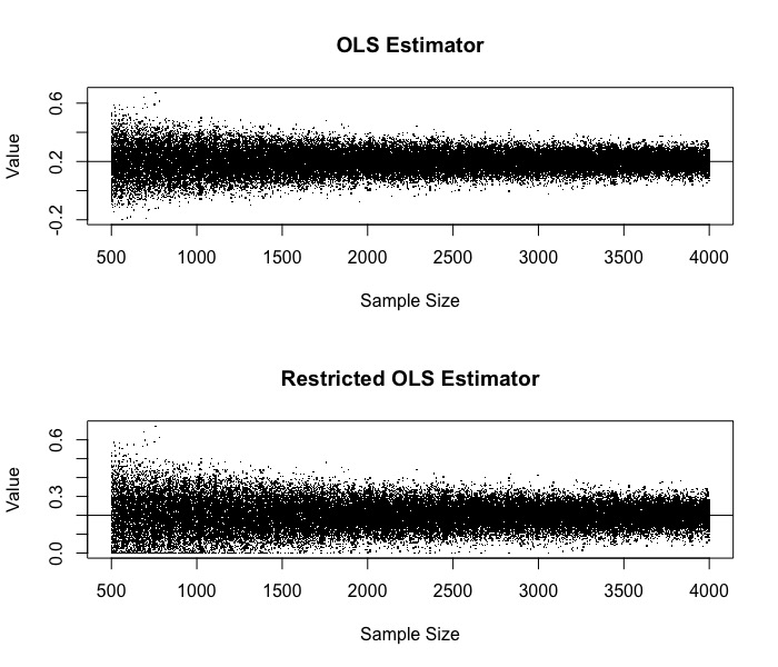
Consistency

Finally, $\hat{\beta}_1^+$ converges to $\hat{\beta}_1$ in probability. This is because since $\hat{\beta}_1 \to \beta_1$ in probability, so eventually $\hat{\beta}_1$ will be positive, and the probability that $\hat{\beta}_1 < 0$ can be ignored. Rigorously,

The second probability is zero for sufficiently small $\epsilon$. The first probability satisfies that

which goes to zero as $n\to\infty$.

This is not so surprising. After all, what we have done is just to drop the estimates that are known to be wrong!

set.seed(64)

beta_1_hat_list <- c()
beta_1_hat_c_list <- c()
x_pos <- c()
for (n in seq(500, 4000, length.out = 500)) {
  for (i in 1:100) {
    beta_0 <- 0.2
    beta_1 <- 0.2
    x <- rnorm(n, mean = 0.2, sd = 1)
    y <- beta_0 + x*beta_1 + rnorm(n, mean = 1, sd = 3)
    
    beta_1_hat <- sum((x-mean(x))*y) / sum(var(x)*(n-1))
    beta_1_hat_c <- max(beta_1_hat, 0)
    
    x_pos <- c(x_pos, n)
    beta_1_hat_list <- c(beta_1_hat_list, beta_1_hat)
    beta_1_hat_c_list <- c(beta_1_hat_c_list, beta_1_hat_c)
  }
}

par(mfrow = c(2, 1))
plot(x_pos, beta_1_hat_list, main = "OLS Estimator", xlab = "Sample Size", ylab = "Value", pch = '.')
abline(h = 0.2)
plot(x_pos, beta_1_hat_c_list, main = "Restricted OLS Estimator", xlab = "Sample Size", ylab = "Value", pch = '.')
abline(h = 0.2)

Extract values from an R data frame in 9 ways

Compared to pandas, subsetting in R is slightly more complicated. Most of the time, we use .iloc and .loc to subset a pandas data frame. (There was also .ix, but luckily, it is deprecated.) So there are only 2 functions to master. However, R has so many different ways to subset a data frame. In fact, there is an exercise in Advanced R:

Brainstorm as many ways as possible to extract the third value from the cyl variable in the mtcars dataset.

I am sure that the readers already know several different ways of doing this (e.g. mtcars[3, "cyl"]). But I will try to come up with as many different solutions as possible by considering the order of subsetting. That is, we can

1. First select the column “cyl”, and then find its 3rd element. Or
2. First select the 3rd row, and the find the “cyl” element. Or
3. Directly find the element.

Directly select the element

The most straightforward solution would be mtcars[3, "cyl"].

Column, then row

A data frame in R is just a list, where its name is just the column name. As a result, we have the following 2 solutions:

1. mtcars$cyl[3]
2. mtcars[["cyl"]][3]

Both $ and [[ ]] are standard way to get elements from a list. Both mtcars$cyl and mtcars[["cyl"]] are atomic vectors.

Another way would be

1. mtcars[, "cyl"][3]

mtcars[, "cyl"] also returns an atomic vector. This is the default behaviour of [, ] when the second index is a single integer/character string, and drop=FALSE is not specified. When drop=FALSE is specified, it maintains the dimension and returns a n-by-1 data frame.

We can also first obtain a “sub-data frame” (instead of an atomic vector), and then proceed. That is,

1. mtcars["cyl"][3, ]
2. mtcars[, "cyl", drop=FALSE][3, ]

Here, mtcars["cyl"] returns a n-by-1 data frame (unlike mtcars[["cyl"]]). As a result, it is incorrect to write mtcars["cyl"][3] because [3] is interpreted as “select the 3rd column” when mtcars["cyl"] has only 1 column.

Row, then column

We can also first select the 3rd row, and then select the “cyl” from that row:

1. mtcars[3, ][, "cyl"]
2. mtcars[3, ][["cyl"]]
3. ` mtcars[3, ]$cyl`

Here mtcars[3, ] returns a 1-by-p data frame, not an atomic vector. This makes sense, since an atomic vector can only contain one type of elements, but different columns of a data frame can be of different types (e.g. factor, numeric). A follow-up question: What does mtcars[3, , drop=TRUE] return? Why?

An interesting bug in the package RandomForest

Environment and a reproducible example

I ran into this interesting bug with the randomForest package in R when I was trying to make some partial dependence plots. I was running R version 3.5.2, and the version of the randomForest package was 4.6.14.

> library(randomForest)
> packageVersion("randomForest")
[1] '4.6.14'

To replicate the bug, run the following codes:

rf_model <- randomForest(x = iris[, colnames(iris) != "Species"], y = iris$Species)

# This works fine
partialPlot(rf_model, iris, x.var = "Sepal.Length")
partialPlot(rf_model, iris, x.var = Sepal.Length)
partialPlot(rf_model, iris, x.var = c("Sepal.Length", "Sepal.Width")[1])

# But this does not work
var_interested <- "Sepal.Length"
partialPlot(rf_model, iris, x.var = var_interested)
# Error in `[.data.frame`(pred.data, , xname) : undefined columns selected

The failure is surprising, and we will find out why it happens.

Getting the source code

To figure out what is going wrong, we need to look at the source code. A common way to do this is to use the print() function.

> print(randomForest::partialPlot)
function (x, ...) 
UseMethod("partialPlot")
<bytecode: 0x7f8f80b01bc8>
<environment: namespace:randomForest>

This does not give us much information. Since the first argument passed to partialPlot() has class randomForest, we try

> print(randomForest::partialPlot.randomForest)
Error: 'partialPlot.randomForest' is not an exported object from 'namespace:randomForest'
> print(randomForest:::partialPlot.randomForest)  # recall the difference between :: and :::

And this will gives us the source code for partialPlot.randomForest(). The first couple of lines read

function (x, pred.data, x.var, which.class, w, plot = TRUE, add = FALSE, 
    n.pt = min(length(unique(pred.data[, xname])), 51), rug = TRUE, 
    xlab = deparse(substitute(x.var)), ylab = "", main = paste("Partial Dependence on", 
        deparse(substitute(x.var))), ...) 
{
    classRF <- x$type != "regression"
    
    if (is.null(x$forest)) 
        stop("The randomForest object must contain the forest.\n")
        
    x.var <- substitute(x.var)
    xname <- if (is.character(x.var)) 
                x.var
            else {
                if (is.name(x.var)) 
                    deparse(x.var)
                else {
                    eval(x.var)
                }
            }
    ...

Apparently, when we write x.var = var_interested, the function does not assign the correct value to xname.

What does substitute() do?

According to the documentation,

substitute() returns the parse tree for the (unevaluated) expression expr, substituting any variables bound in env

Substitution takes place by examining each component of the parse tree as follows: If it is not a bound symbol in env, it is unchanged. If it is a promise object, i.e., a formal argument to a function or explicitly created using delayedAssign(), the expression slot of the promise replaces the symbol. If it is an ordinary variable, its value is substituted, unless env is .GlobalEnv in which case the symbol is left unchanged…

Although the explanation is terse, we only need to pay attention to the bolded sentence, since in our case, substitute() is used inside a function. For any expression supplied to the argument x.var, substitue() will simply let x.var be that expression. Consider the following example.

f <- function(x.var) {
    print(pryr::ast(x.var))  # show the parse tree
    x.var <- substitute(x.var)
    print(x.var)
    print(class(x.var))

}

> f(x.var = "Sepal.Length")
\- `x.var 
NULL
[1] "Sepal.Length"  # "Sepal.Length" is supplied to x.var
[1] "character"  # And obviously, "Sepal.Length" is character

> f(x.var = Sepal.Length)
\- `x.var 
NULL
Sepal.Length  # Sepal.Length is supplied to x.var, without quotes
[1] "name"  # Sepal.Length is not character since there is no quote. It's just a name.

So why does the function fail if we assign the quoted names "Sepal.Length" to var_interested?

> var_interested <- "Sepal.Length"
> f(x.var = var_interested)
\- `x.var 
NULL
var_interested
[1] "name"

Let’s be a little bit more careful here. We first assigned "Sepal.Length" (which is a character) to the variable var_interested. Then, we assigned var_interested to the argument x.var. You might expect substitute(x.var) to return "Sepal.Length", but this is not the case! substitute() will only substitute x.var with whatever is assigned to it (in this case, it’s the variable name var_interested), not the underlying evaluated value. So when we enter the if-else statements, since x.var is not character, but a name, xname <- deparse(x.var) is executed. Now, the function will look for a column with name “var_interested”, and of course it cannot find it. In conclusion, we have this bug because the author assumed that if the user pass something without quotes to x.var, it is always the name of the column without quotes.

But why would this example work?

partialPlot(rf_model, iris, c("Sepal.Length", "Sepal.Width")[1])

When we call substitute(x.var), it first looks at the parse tree of the expression x.var, which is just x.var itself. Then it tries to replace it with the expression c("Sepal.Length", "Sepal.Width")[1]. Recall that any R expression has 4 components: call, constant, pairlist, and names. The expression c("Sepal.Length", "Sepal.Width")[1] is a call, since we are calling the function c() first, then the subsetting function []. To verify this, we can type

> is.call(substitute(c("Sepal.Length", "Sepal.Width")[1]))
[1] TRUE
> is.name(substitute(c("Sepal.Length", "Sepal.Width")[1]))
[1] FALSE

Since it is not a character, nor a name, it gets evaluated directly in the if-else statements, thus giving x.var the correct value (which is "Sepal.Length").

Final thoughts: should we encourage non-standard evaluation?

This is a strange bug, and it requires good understanding of advanced R to debug. However, if we require user to supply a character string in the first place, then we would have not encounter this bug. For example, a common approach is to raise an error if is.character(x.var) returns FALSE.

Non-standard evaluation can be handy. Yet my personal opinion is that, under many circumstances, it only saves us from typing many quotes. For users coming from a different programming language (e.g. Python, Java), non-standard evaluation can cause more confusions than benefit.