A simple restricted OLS estimator

27 Feb 2020 [ ]

Last week, I attended a presentation on how to estimate large loss trend. The presentation was interesting, and raised the following question: how to incorporate prior knowledge into estimation, so that the uncertainy of the model can be reduced? This is, of course, a very important and widely-studied question. In fact, one reason why Bayesian statistics attract people is that it can incorporate prior knowledge into the model.

However, since the presentation used a frequentist model, and I am more comfortable with frequentist statistics, I was inspired to think about the following simple question, which is an interesting small exercise:

Question

Consider a simple linear regression model $y_i = \beta_0 + \beta_1 x_i + \epsilon_i$ where the commonly seen assumptions about regression model hold. Here, $\beta_1 > 0$. Denote the OLS estimator of $\beta_1$ as $\hat{\beta}_1$, and define $\hat{\beta}_1^+ = \max \{0, \hat{\beta}_1 \}$. Compare the performance of $\hat{\beta}_1$ and $\hat{\beta}_1^+$.

In other words, since we already know that $\beta_1$ cannot be negative, we will “shrink” the OLS estimator we get $\hat{\beta}_1$ to zero if it is negative.

Unbiasedness

By doing so, obviously we no longer have an unbiased estimator. This is simply because, well, $\hat{\beta}_1$ is unbiased and $\hat{\beta}_1 \ne \hat{\beta}_1^+$. In fact, since $\mathbb{P}\{ \hat{\beta}_1^+ \le t\} = 0$ when $t < 0$, we can actually find an expression for the bias of $\hat{\beta}_1+$.

\[\text{bias}\left( \hat{\beta}_1^+\right) = \mathbb{E}\left[ \hat{\beta}_1^+ \right] - \beta_1 = \int_0^\infty b\cdot f_{\hat{\beta}_1} \left(b\right) \,db - \beta_1\]

where $f_{\hat{\beta}_1}$ is the probability density of $\hat{\beta}_1$, the OLS estimator. This has an interesting indication: If $\hat{\beta}_1$ has large variance, than the bias will be large, too. If $\hat{\beta}_1$ has smaller variance, than the bias will not be as big. This makes intuitive sense because if $\hat{\beta}_1$ has smaller variance, than there is a smaller chance for it to be below zero (Remember, we know that $\beta_1 > 0$ and $\hat{\beta}_1$ estimates $\beta_1$ with no bias).

Variance

By sacrificing unbiasedness, hopefully we would get something in return. This is indeed the case since $\hat{\beta}_1^+$ has smaller variance. To prove this, simply notice that

\[\hat{\beta}_1 = \max \{ \hat{\beta}_1, 0 \} + \min \{ \hat{\beta}_1 , 0\} =: \hat{\beta}_1^+ + \hat{\beta}_1^-\]

We have \(\text{Var}\left[ \hat{\beta}_1\right] = \text{Var}\left[ \hat{\beta}_1^+\right] + \text{Var}\left[\hat{\beta}_1^-\right] + 2\text{Cov}\left[ \hat{\beta}_1^+, \hat{\beta}_1^-\right]\)

It suffices to prove that the covariance term is non-negative. This is conceivably true, since when $\hat{\beta}_1^+$ goes from zero to some positive number, $\hat{\beta}_1^-$ goes from negative to zero, thus moving in the same direction. Formally,

\[\text{Cov}\left[ \hat{\beta}_1^+, \hat{\beta}_1^-\right] = \mathbb{E}\left[ \hat{\beta}_1^+ \hat{\beta}_1^-\right] - \mathbb{E}\left[\hat{\beta}_1^+\right] \mathbb{E}\left[ \hat{\beta}_1^-\right] = - \mathbb{E}\left[\hat{\beta}_1^+\right] \mathbb{E}\left[ \hat{\beta}_1^-\right] \ge 0\]

We can also run a small numerical simulation.

set.seed(64)

beta_1_hat_list <- c()
beta_1_hat_c_list <- c()

for (i in 1:1000) {
  beta_0 <- 0.2
  beta_1 <- 0.2
  x <- rnorm(1000, mean = 0.2, sd = 0.8)
  y <- beta_0 + x*beta_1 + rnorm(1000, mean = 1, sd = 5)
  
  beta_1_hat <- sum((x-mean(x))*y) / sum(var(x)*999)
  beta_1_hat_c <- max(beta_1_hat, 0)
  
  beta_1_hat_list <- c(beta_1_hat_list, beta_1_hat)
  beta_1_hat_c_list <- c(beta_1_hat_c_list, beta_1_hat_c)
}

par(mfrow = c(1, 2))
hist(beta_1_hat_list, main = "OLS Estimator", xlab = "Value", breaks = 20)
abline(v = mean(beta_1_hat_list), col = "blue", lwd = 4)
hist(beta_1_hat_c_list, main = "Restricted OLS Estimator", xlab = "Value", breaks = 15)
abline(v = mean(beta_1_hat_c_list), col = "blue", lwd = 4)

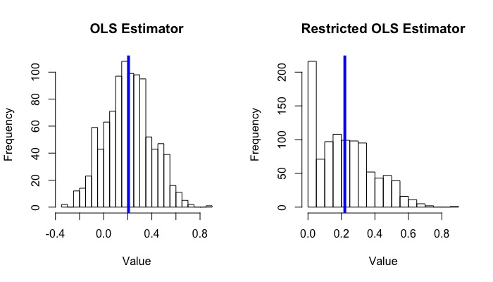
The average of 1000 $\hat{\beta}_1^+$ is around 0.220, while the average of $\hat{\beta}_1$ is around 0.207.

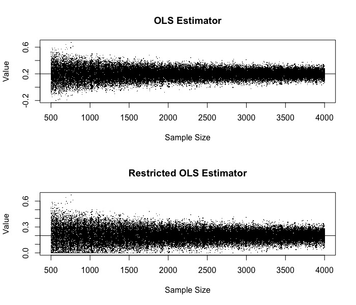
Consistency

Finally, $\hat{\beta}_1^+$ converges to $\hat{\beta}_1$ in probability. This is because since $\hat{\beta}_1 \to \beta_1$ in probability, so eventually $\hat{\beta}_1$ will be positive, and the probability that $\hat{\beta}_1 < 0$ can be ignored. Rigorously,

\[\mathbb{P}\left\{ | \max \{ \hat{\beta}_1, 0\} - \beta_1 | > \epsilon \right\} = \mathbb{P}\left\{ |\hat{\beta}_1 - \beta_1 | > \epsilon , \hat{\beta}_1 > 0\right\} + \mathbb{P}\left\{ |\beta_1| > \epsilon, \hat{\beta}_1 < 0\right\}\]

The second probability is zero for sufficiently small $\epsilon$. The first probability satisfies that

\[\mathbb{P}\left\{ |\hat{\beta}_1 - \beta_1 | > \epsilon , \hat{\beta}_1 > 0\right\} \le \mathbb{P}\left\{ |\hat{\beta}_1 - \beta_1 | > \epsilon \right\}\]

which goes to zero as $n\to\infty$.

This is not so surprising. After all, what we have done is just to drop the estimates that are known to be wrong!

set.seed(64)

beta_1_hat_list <- c()
beta_1_hat_c_list <- c()
x_pos <- c()
for (n in seq(500, 4000, length.out = 500)) {
  for (i in 1:100) {
    beta_0 <- 0.2
    beta_1 <- 0.2
    x <- rnorm(n, mean = 0.2, sd = 1)
    y <- beta_0 + x*beta_1 + rnorm(n, mean = 1, sd = 3)
    
    beta_1_hat <- sum((x-mean(x))*y) / sum(var(x)*(n-1))
    beta_1_hat_c <- max(beta_1_hat, 0)
    
    x_pos <- c(x_pos, n)
    beta_1_hat_list <- c(beta_1_hat_list, beta_1_hat)
    beta_1_hat_c_list <- c(beta_1_hat_c_list, beta_1_hat_c)
  }
}

par(mfrow = c(2, 1))
plot(x_pos, beta_1_hat_list, main = "OLS Estimator", xlab = "Sample Size", ylab = "Value", pch = '.')
abline(h = 0.2)
plot(x_pos, beta_1_hat_c_list, main = "Restricted OLS Estimator", xlab = "Sample Size", ylab = "Value", pch = '.')
abline(h = 0.2)