Some thoughts on "trend" of time series

Everyone agrees that you should care about the “trend” in your time series. For example, it is a common practice to “decompose” your time series into 3 components: trend, seasonality, and randomness. You can do this easily in R using decompose(). However, decomposition might not be as useful as you might think, and sometimes it only confirms your bias.

Data scientists use the term “trend” loosely. Most of the time, when they say “I see an upward trend”, they mean exactly that: The plot goes upward. If a data scientist, with this assumption, use decompose() to decompose the time series at hand, he will only see a smoothed version of the original time series.

As a result, he might be tricked into thinking “there is indeed an upward trend, and statistics (?) just proved it!”. But consider the following two time series:

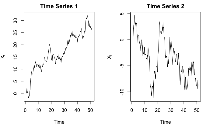
Obviously, in the first graph we see an upward trend, and in the second graph we see a downward trend. Right?

In fact, they are both simulated from $Y_t = Y_{t-1} + \epsilon_t$ where $\epsilon_t \sim N(0,1)$, and $Y_1 = 0$. So $\mathbb{E}\left[X_t\right] = 0$ for all $t$. The observed $X_t$’s indeed go up, but it would be quite ridiculous to say $X_t$ has an upward trend when we, in fact, know that $\mathbb{E}\left[X_t\right] = 0$.

Here is the code used to generate those two series

set.seed(7)

simulate_randomwalk <- function(X_init = 0, noise_mean = 0, noise_var = 1, n_step) {
  ret = c(X_init)
  for (i in 1:n_step) {
    ret <- c(ret, ret[length(ret)] + rnorm(1, noise_mean, noise_var))
  }
  ts(ret)
}

par(mfrow = c(1, 2))
ts_1 <- simulate_randomwalk(n_step = 200) %>% ts(frequency = 4)
plot(ts_1, ylab = expression(X[t]), main = "Time Series 1")

ts_2 <- simulate_randomwalk(n_step = 200) %>% ts(frequency = 4)
plot(ts_2, ylab = expression(X[t]), main = "Time Series 2")

Simply by looking at the shape of the curve does not benefit us much. In practice, we should use context of the data and existing domain knowledge to help us determine if there is any trend or not. In fact, this probably is the only way because we cannot prove there exists a trend mathematically. For example, consider the following example:

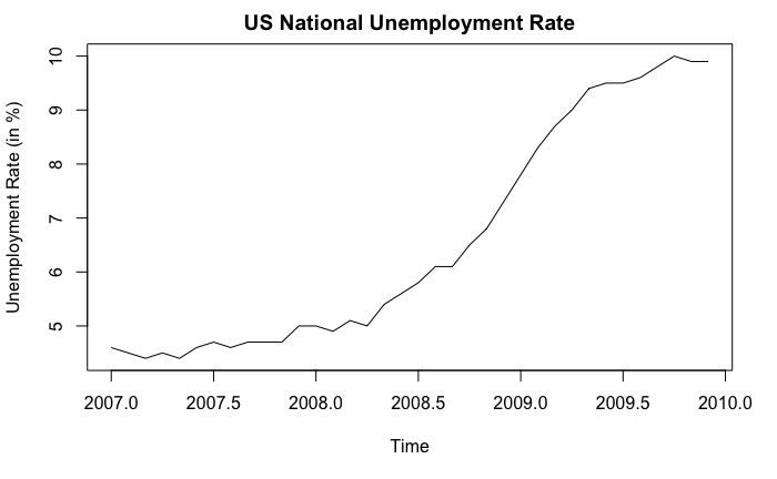
In this example, we can confidently say that an upward trend exists, not because the curve goes up, but because we know what the curve stands for: unemployment rate. From economic theories (or common sense), a 5% increase in unemployment rate cannot possibly be due to “randomness” and is considered to be very significant. Also, if we look at the x-axis, we know that the upward trend is supported by the financial crisis happened around 2008.

To summarize, as Jonathan D. Cryer and Kung-Sik Chan put in their book Time Series Analysis With Applications in R,

“Trends” can be quite elusive. The same time series may be viewed quite differently by different analysts.