Calculating exact multiplicative calibration using SQL

This post will talk about what exact multiplicative calibration (EMC) is, and how to calculate this metric using SQL.

What is exact multiplicative calibration?

In the context of predictive modeling, we often think about prediction error from two different perspectives: bias and variance. Roughly speaking, bias is about if our predictions are systematically larger or smaller than the ground truth.

One way to think about bias is this: Given a set of predictions, is it possible to make it more accurate (defined using some loss function such as MSE or quantile loss) by simply applying the same adjustments to all predictions? (Well, you can always multipley each forecast by a different constant to make it perfect! But it’s trivial.) For example, if we add a constant $c$ or multiply a non-zero constant $k$ to all predictions, does that give us more accurate predictions?

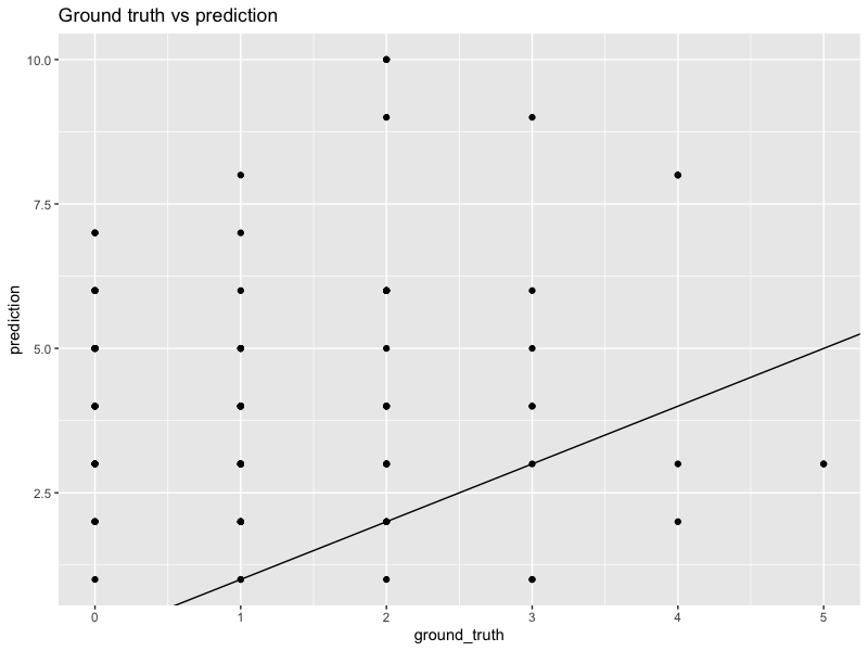
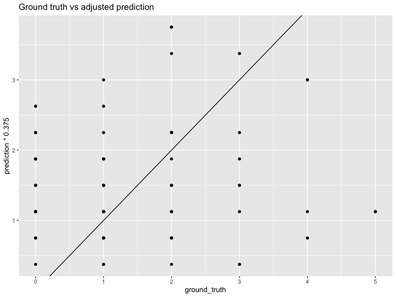
In the example above, we see that the original forecasts are over-biased. They have a higher MSE of $13.8$, too. However, if we multiply every forecast by a constant $0.375$, then the calibration looks much better. The MSE also decreases to $2$.

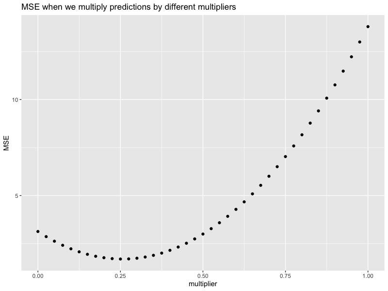
So this ia a better forecast. The natural follow-up question is, then, can we find an even better forecast? That is a fair question, and $0.375$ is no magic number. Obviously we should look for a constant that’s smaller than 1 to adjust the over-biasness. We can do a grid search over the interval $(0, 1)$ with step size $0.025$.

Below is a plot showing different MSEs when we multiply predictions with different multiplier. It is quadratic (why?), and we see that multiply all predictions by $0.25$ will give us the smallest MSE, which is around $1.69$.

Formalizing the idea of grid search, exact multiplicative calibration (EMC) for this problem is a constant $c$ such that $\text{MSE} (\mathbf{y}, c\cdot \hat{\mathbf{y}})$ is minimized.

How to calculate EMC using SQL?

Finding EMC analytically for a given metric can be difficult. Even for MSE, the analytical solution can be somewhat complicated. In practice, grid search is a powerful idea and can be used for other metrics such as MAE or quantile loss.

Data scientists often work with SQL tables. How do we calculate EMC using SQL? The idea is to first create a table of multiplier candidates:

DECLARE
  smallest_m  FLOAT := 0.1;
  largest_m   FLOAT := 2.0;
  search_step FLOAT := 0.01;
-- We do a grid search over (0.1, 2.0) with step size of 0.01

BEGIN
  -- Create a 1-column table with all possible multipliers for grid search.
  DROP TABLE IF EXISTS grid_search_table;
  CREATE TEMP TABLE grid_search_table (
    m FLOAT
  );
  WHILE smallest_m <= largest_m
    LOOP
      INSERT INTO grid_search_table VALUES (smallest_m);
      smallest_m = smallest_m + search_step;
    END LOOP;

Once we have this table, we can cross join it with another table prod_tbl containing both predictions as well as ground truth. In practice, we usually want to look at metric and EMC of certain subgroups. For example, if we are predicting housing prices, we might want to know if predictions for single family house are better-calibrated than the ones for townhomes. So we apply GROUP BY on those fields. The resulting table main_calc_tbl will be a much larger table than prod_tbl due to the CROSS JOIN.

DROP TABLE IF EXISTS main_calc_tbl;
CREATE TEMP TABLE main_calc_tbl AS (
  SELECT
    prod_tbl.house_type,
    prod_tbl.prediction,
    prod_tbl.target,
    grid_search_table.m,
    -- We should also calculate the loss metric in this step.
    -- We calculate both the actual MSE as well as hypothetical MSE when predictions
    --   are multiplied by the multiplier m.
    AVG(POWER(prod_tbl.target - prod_tbl.prediction, 2)) AS actual_mse,
    AVG(POWER(prod_tbl.target - prod_tbl.prediction * grid_search_table.m, 2)) AS mse,
  FROM prod_tbl CROSS JOIN grid_search_table
  GROUP BY prod_tbl.house_type
);

Finally, we need to find which multiplier m gives us the smallest loss. To do this, we create a CTE with minimized loss, and then use this CTE to get the final result.

DROP TABLE IF EXISTS emc_result;
CREATE TEMP TABLE emc_result AS (
  WITH h AS (
    SELECT house_type,
           MIN(actual_mse) AS actual_mse,  -- This doesn't really do anything, just keeping the actual MSE.
           MIN(mse)        AS mse  -- Minimum of all MSEs, each of which is based on a different multiplier.
    FROM main_calc_tbl
    GROUP BY house_type)

  SELECT house_type,
         h.actual_mse,
         h.mse           AS minimized_mse,
         main_calc_tbl.m AS emc
  FROM h
    JOIN main_calc_tbl USING (house_type, mse)
  );

Double machine learning for causal inference

Recently I have been working on causal inference problems. Mainly I am trying to understand how many more units of sales Amazon can expect if we are able to offer faster delivery speed. This is a typical causal inference problem, where the treatment would be the faster delivery speed, and the control would be the slower delivery speed. Upon research, I was introduced to this interesting method called “double machine learning”. This post will document some of the learnings I have had so far.

Notation and Setup

Following convention, let’s denote the treatment indicator for each unit $i$ as $T_i$. In the case where there is only one possible treatment, we write $T_i = 0$ if unit $i$ receives the control, and $T_i = 1$ if unit $i$ receives the treatment. We follow the potential outcome framework, so let $D_i(0)$ be the potential outcome of unit $i$ under control, and $D_i(1)$ be the potential outcome of unit $i$ under treatment.

Now, the observed outcome $D_i$ is

Obviously, observed outcome depends on the treatment it receives. For a fixed unit $i$, $D_i$ is either $D_i(0)$ or $D_i(1)$.

We can also write the observed outcome as

In other words, we can express the observed outcome in terms of the individual treatment effect (ICE), $D_i(1) - D_i(0)$. This quantity is very difficult to estimate, and might not be needed after all.

Double machine learning

Let’s talk about how double machine learning works now. Again, we have two possible scenarios for each unit: control vs treatment. The treatment assignment of unit $i$ (i.e. whether unit $i$ is under control or not) itself is random, and we denote it as $T_i$. Once the treatment assignment is fixed, the potential outcomes $D_i(0)$ and $D_i(1)$ are also random, and depend on a set of covariates $X_i$. In other words, $D_i(0), D_i(1)$ as well as $T_i$ are all random variables.

Dropping the index $i$, we assume that we can write $D$ in terms of conditional expectations plus a white noise. That is,

Let’s take conditional expectation on both sides. When we condition on $X$, terms like $\mathbb{E}[\cdot \mid X]$ behave like constants and can be pulled out directly. So

But since it’s an indicator function in the expectation, the conditional expectation $ \mathbb{E}[\mathbf{1}\{{T=1}} \mid X] $ really is just the conditional _probability of receiving treatment instead of control. Let $p_T(t) = \mathbb{P}\left[T=t\right]$. So let’s rewrite it as

Here comes the interesting part. We can group terms by their treatment status. Under the ignorability assumption, we finally arrive at

We call this quantity mean outcome and denote it as $m(X)$, and the reason should be clear. The conditional expectation of outcome $\mathbb{E}\left[D\mid X\right]$ can be viewed as an weighted average. We weigh each potential outcome by their propensity score (i.e. probability of receiving the corresponding treatment).

Subtract mean outcome from both sides of equation (2) and recall that $p_T(0) + p_t(1) = 1$, we have

Assuming that $m(\cdot)$ and $p_T(\cdot)$ are known, then there is a natural estimator for $\mathbb{E}\left[D(1) - D(0)\right]$. Namely, we can run a regression of $ D_i-m(X_i) $ with respect to $ [\mathbf{1}_{{T_i=1}} - p_{T_i}(1)] \phi(X)$ where $\phi(\cdot)$ is some function. For simplicity, we will assume that the lift is linear in covariate, even though this is not required to achieve good asymptotic consistency. That is,

In practice, $m(\cdot)$ and $p_T(\cdot)$ have to be estimated. In terms of model class, we have many choices. Neural networks can be used to model the mean outcome $m(\cdot)$, while logistic regression can be used to model propensity score $p_T(\cdot)$.

The final regression will yield a set of coefficients $\hat{\beta}$. In production, we simply need to multiply the covariates with $\hat{\beta}$ to generate lift estimates.

Some technical discussions on behaviour of decision tree splitting (cont'd)

Swapping elements to reduce $SS$

Although we omit the proof, we show how to reduce $SS$ by swapping using a demo. Let’s take $L = \{1,3\}, R = \{2,4,5\}$ as an example.

SS <- function(v) PreciseSums::fsum((v - mean(v))^2)

L_array <- c(1,3)
R_array <- c(2,4,5)

while (TRUE) {
  cat("------------------------------------\n")
  # Make sure L has smaller average
  if (mean(L_array) > mean(R_array)) {
    tp <- L_array
    L_array <- R_array
    R_array <- tp
  }
  
  ss_before_swap <- SS(L_array) + SS(R_array)
  cat("Before swapping SS: ", ss_before_swap, "\n")
  cat("Input: ", L_array, "░", R_array, "\n")
  
  L_array <- sort(L_array)
  R_array <- sort(R_array)
  
  cat("Sort:  ", L_array, "░", R_array, "\n")
  
  # Check if max(L_array) <= min(R_array). If not, swap them
  if (L_array[length(L_array)] > R_array[1]) {
    cat("Swap ",L_array[length(L_array)], " and ", R_array[1],"\n")
    right_most <- L_array[length(L_array)]
    left_most <- R_array[1]
    L_array[length(L_array)] <- left_most
    R_array[1] <- right_most
    
    ss_after_swap <- SS(L_array) + SS(R_array)
    
    cat("\nOutput: ", L_array, "░", R_array, "\n")
    cat("After swapping SS:  ", ss_after_swap, "\n")
  } else {
    cat("Paused. Condition L ⊲ R met.\n")
    break
  }
}

Because there are only 15 partitions for $\{1,2,3,4,5\}$, we can even plot all of them.

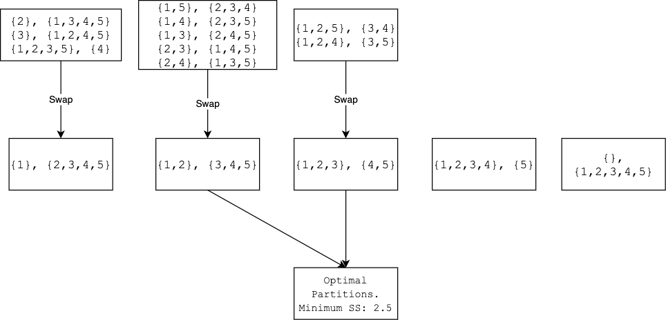
In conclusion, to find the optimal partition, it is best to work with the sorted $\mathbf{y}$. By going through all $n$ possible partitions, we are guaranteed to minimize the impurity $SS(L) + SS(R)$. If $\mathbf{y}$ is not sorted, then there is no guarantee.

Notice that if there are $l$ elements in the optimal left partition, then there are $l!(n-l)!$ possible permutations of $\mathbf{y}$ that guarantees an optimal partition if you do a linear scan. So, if $\mathbf{y}$ is in a random order, then the chance of finding the optimal partition using a linear scan on $\mathbf{y}$ is $\frac{l!(n-l)!}{n!}$. This is extremely small.$^{1}$.

Find $\mathbf{x}$ that is close to $\mathbf{y}$.

Built upon what we have analyzed, we can see why the idea “find the $\mathbf{x}$ strongly correlated with $\mathbf{y}$” could be right or wrong. Intuitively, if $\mathbf{x}$ and $\mathbf{y}$ has exactly the same order, then we will sort $\mathbf{y}$ when we sort $(\mathbf{x}_i, \mathbf{y})$ together using $\mathbf{x}_i$. As we have explained, an ordered $\mathbf{y}$ will guarantee us the optimal partition.

But we have also seen that an unordered $\mathbf{y}$ might give you the minimum $SS$, too. We just need to make sure that after we sort $(\mathbf{x}_i, \mathbf{y})$ together using $\mathbf{x}_i$, one of the $(L, R)$ partition is the same as the optimal one, up to permutation within $L$ and $R$ respectively.

Indeed, the following statements are both wrong.

An incorrect statement: Given features $X_1,\cdots,X_n$ and a response $Y$, a decision tree always chooses the $X_i$ that maximizes its Pearson correlation with $Y$.

Another incorrect statement: Given features $X_1,\cdots,X_n$ and a response $Y$, a decision tree always chooses the $X_i$ that maximizes its Spearman’s correlation with $Y$.

Here are the counterexamples.

# Counterexample to statement 1
Ckmeans.1d.dp::Ckmeans.1d.dp(c(1,2,3,4,5,6), k = 2)

train_df <- data.frame(X1 = c(1,3,4,5,6,7),
                       X2 = c(1,4,5,6,7,8),
                       Y  = c(1,2,3,4,5,6))

stats::cor.test(train_df$X1, train_df$Y, method = 'spearman')$estimate
stats::cor.test(train_df$X2, train_df$Y, method = 'spearman')$estimate

# Counterexample to statement 2
train_df <- data.frame(X1 = c(1,2,6,3,4,5),
                       X2 = c(3,1,2,6,5,4),
                       Y  = c(1,2,3,4,5,6))

In counterexample 2, $\mathbf{x}_1$ has higher Spearman’s correlation with $\mathbf{y}$ than $\mathbf{x}_2$ (0.657 versus 0.6). However, if we use $\mathbf{x}_1$ to sort our $\mathbf{y}$ and look for the best partition, the minimum $SS$ will be $5.5$. On the contrary, if we use $\mathbf{x}_2$, the minimum SS is $4$, which is better.

Going back to the original question

So, going back to the original question,

Is there any smarter way to find the best feature $\mathbf{x}$, without going through all the features? If not, is there any smarter way to understand the whole process at least?

At least for now, the answer is “no”. But it was a fun exercise.

Footnotes:

$^{1}$ We implicitly assume that there is only one optimal partition. This is not the case. For example, $\{1,2,3,4,5\}$ have two different partitions both giving the smallest $SS$, 2.5. Is it possible to have more than 2 partitions such that they all give the smallest $SS$?

I appreciate my friend Tai Yang for taking time to discuss this problem with me.

Some technical discussions on behaviour of decision tree splitting

How does a regression decision tree choose on which feature to split?

This is like Data Science 101, so I will not go through the details. You can read [1] to refresh the memory. Here is the rough idea:

• Do the following steps for every feature $\mathbf{x}_1,\cdots,\mathbf{x}_p$
  • Sort $(x_i, y)$ in non-descending order of $x_i$. Call the sorted pair $(x_i’, y’)$. Note that for different $x_i$’s we will get different $y_i’$.
  • Divide $\mathbf{y}’$ (i.e. the sorted $\mathbf{y}$) into a left part $L = \{y_i’ \le y_1’\}$ and a right part $R = \{y_i > y_1’\}$, and compute something called impurity. For regression tree, a commonly used impurity measure is $SS(L) + SS(R)$. Here, $SS$ is the sum of squared error, defined as $SS(x_1,\cdots,x_n) = \sum_{i=1}^n (x_i - \bar{x}_n)^2$, where $\bar{x}_n$ is the sample average.
  • Repeat the previous step, but change $y_1’$ to $y_2’, y_3’, \cdots, y_n’$.
  • We have examined $n$ different partitions. Keep the one that gives the smallest impurity $SS(L) + SS(R)$
• Now we have the smallest impurity $SS(L) + SS(R)$ for each feature. Choose the feature with the smallest overall impurity.

The question I was interested in was this:

Question 0: Is there any smarter way to find the best feature $\mathbf{x}$, without going through all the features? If not, is there any smarter way to understand the whole process at least?

If you examine the algorithm, obviously the magic happens when we create partition $L$ and $R$ on the sorted vector $\mathbf{y}’$. To get to the essence of the problem, let’s ignore $\mathbf{x}_i$ for now, and think about the following problem:

Question 1: Given a vector $\mathbf{y}$, and re-order it (or equivalently, permute it) to get another vector $\mathbf{y}’ := \pi(\mathbf{y})$. We then partition the re-ordered vector $\mathbf{y}’$ into a left part $L$ and a right part $R$. If we want to minimize $SS(L) + SS(R)$, how should we re-order $\mathbf{y}$ (i.e. what is the optimal $\pi^*(\cdot)$)? How should we partition it after that?

Note that we are only allowed to cut the array in half from the middle. For example, if we have $\mathbf{y} = \{1, 2, 3, 4\}$, we can’t say that $L = \{1, 3\}$ because there is a $2$ between them.

For simplicity, let’s define order function $o(\mathbf{x})$. This is the same as order() in R. For example, $o([5,2,7]) = [2,1,3]$. If we can answer Question 1, then we can think of Question 0 in this way:

There is a permutation $\pi^*$ such that if you partition $\pi^*(\mathbf{y})$ into a left part and a right part, you can minimize $SS(L) + SS(R)$. To find the best feature, we just need to find the feature $\mathbf{x}^*$ such that $|o(\mathbf{x}^*) - o(\pi(\mathbf{y}))|$ is as small as possible.

Or at least that’s what I thought…

How to find the best partition if $\mathbf{y}$ is sorted already? (Answer: Brute force)

I started with a seemingly easier question: Assume $\mathbf{y}$ is already sorted. Is there any analytical way to find the optimal split point (Note that we can always just scan through all $n$ possibilities)? Formally,

Question 2: Assume $\mathbf{y} = (y_1, y_2, \cdots, y_n)$ is sorted in ascending order. We want to divide $\mathbf{y}$ into a left part $L = \{y \le y_s\}$ and a right part $R = \{y > y_s\}$. How to find a $y_s$ that minimizes $SS(L) + SS(R)$?

At first, I thought sample average and sample median were two promising candidates. Intuitively (at least to me), if we want to make $SS(L) + SS(R)$ small, then the points within each group should be close to each other. As a result, we probably shouldn’t put sample maximum and minimum in the same group.

And indeed, for many samples, the best splitting point $y_s$ is the median or the mean. For example, if $\mathbf{y} = \{1, 2, 3\}$, then we should split it into $L=\{1,2\}$ and $R =\{3\}$. Another good example is $\mathbf{y} = \{1, 2, 3, 4\}$. Here, $y_s = 2$, which is a median.

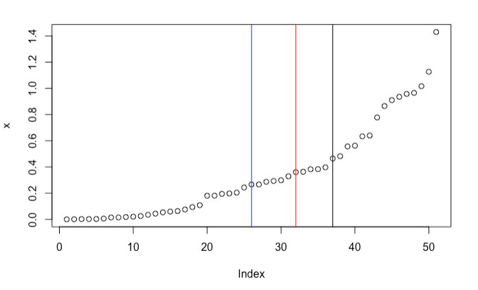
But it’s also easy to find counterexamples. Consider $\mathbf{y} = \{1, 3, 6, 8, 10\}$. It turns out that the best split point is $y_s = 3$. This is neither mean nor median. In fact, sometimes it’s not even close to the “center” of the sample. In the following example, the best split point is the black vertical line. It is quite far from the sample median (in blue) and the sample average (in red).

It seems that there is no analytical solution. You might not be surpried. After all, this is a special case of the more difficult $k$-means clustering problem. Here, we are dealing with a 1-dimensional 2-means clustering problem. For 1-dimensional $k$-means clustering, you can use dynamic programming to find a global optimizer. See referenece [2] for details.

In conclusion, even when $\mathbf{y}$ is sorted, there is no analytical way to find the best split $y_s$. We can always linearly scan through it. So that’s not too bad.

Can I find the best partition on unsorted $\mathbf{y}$? (Answer: In most cases, no)

In general, $\mathbf{y}$ will not be sorted. In such cases, we can still scan the whole thing, and find the best partition for that specific ordering. But how do we know if it is the best one among all possible partitions? See the following example:

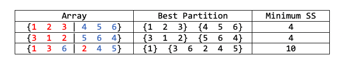
If we are given the third array, we will find that $\{1\}, \{3,6,2,4,5\}$ is the best partition. But it is not the best one globally.

In order to tackle the situation, let’s notice a few things. Let $\mathbf{y}$ be in any order, and $L, R$ be any of its $n$ left/right partitions. We can categorize $(L, R)$ into 2 types:

1. Type I: $\max(L) \le \min(R)$. For example, $L = \{3,2,1\}, R = \{4,6,5\}$. In such case, we write $L \lhd R$.
2. Type II: $\max(L) > \min(R)$. For example, $L = \{1,2,4\}, R = \{3,6,5\}$.

Adopting this view, we immediately conclude the following:

1. If $\mathbf{y}$ is sorted, then every partition $(L, R)$ satisfies that $L \lhd R$.
2. If $\mathbf{y}$ is not sorted, then some of its partitions might still satisfies that $L \lhd R$.

Let’s go back to this example:

The first array is already sorted. No matter how you split it in half, you always end up with $L \lhd R$. The second array is not sorted, but $L = \{3, 1, 2\}, R = \{5, 6, 4\}$ still satisfies $L \lhd R$. However, if we split the second array into $\{3\},\{1,2,5,6,4\}$, then the condition is not satisfied, since $3 > 1$.

Here comes the main result.

Let $\mathbf{y}$ be in any order, and $(L, P)$ be any partition. Assume $\mean(L) < \mean(R)$. As long as $L \lhd R$ does not hold, we can switch $\max(L)$ and $\min(R)$ to make $SS(L) + SS(R)$ smaller. In other words, $L \lhd R$ is a necessary (but not sufficient) condition to minimize $SS(L) + SS(R)$.

The implication, however, is this: If you want to find the best $(L, R)$ globally, you should always start with a sorted $\mathbf{y}$. Because only a sorted $\mathbf{y}$ can guarantee that $L \lhd R$, which is a necessary (but not sufficient) condition for minimizing $SS$.

To be continued in the next post.

References

1. https://scikit-learn.org/stable/modules/tree.html#regression-criteria
2. https://journal.r-project.org/archive/2011-2/RJournal_2011-2_Wang+Song.pdf

How useful are PDP's to analyzing time series data?

How useful are PDP’s to analyzing time series data? If you only care about forecast, then there is literally nothing stopping you from doing anything (e.g. “changing the card”). If you mainly care about extracting insights and valid statistical inference, however, they are as useful (or useless) as the coefficients and p-value’s of a linear regression model. A good starting point would be some classical statistical methods (e.g. VAR model) instead of LightGBM.

What is partial dependence plot (PDP)?

Assume the data is generated by some model $Y = f(X_1, \cdots, X_n)$. The partial dependence of $Y$ on $X_i$ is defined as $g(X_i = x) = \mathbb{E}[ f(X_1,\cdots,X_i = x, \cdots,X_n)]$. In other words, it tells you when $X_i = x$, what will predicted $Y$ be in expectation. Note that, in practice, we rarely know the actual DGP. As a result, we use sample average to estimate PDP and almost always get a wiggly curve. For details on PDP, see reference [1].

Here is a very simple example. Assume that $Y = 0.3 X_1 + 0.7 X_2 + \epsilon$, where $X_1, X_2,$ and $\epsilon$ are all normally distributed with mean $2$. What does the PDP of $X_1$ look like? Following the definition, we see that the PD function is just $g(x) = 0.3x + 0.2 \times 2 + 2 = 0.3x + 2.4$. It’s just a straight line.

Here we have our first important takeaway: For linear regression model, PDP and coefficient estimates are “the same thing”. As a result, PDP is reliable if and only if coefficient estimates are reliable.

But OLS coefficient estimates are often not reliable for time series

It is widely known that running OLS on non-stationary time series might give you unreliable results (i.e. spurious regression). For more details, see page 9 of reference [2]. As a result, its PDP’s are not reliable either.

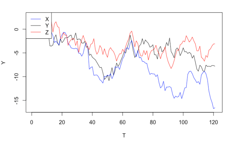
For simplicity, assume we have three time series $X_t, Z_t$ and $Y_t$ that all seem to be “trending downwards”. We want to decide if $X_t$ and/or $Z_t$ are “related to” $Y_t$. Is it possible to figure out by using linear regression? For example, can we rely on coefficient estimate/confidence interval?

The answer is no. Let’s simulate three independent random walks (note: random walks are non-stationary). From the graph, it seems that all of them are trending downwards, which may trick us to believe that they are related to each other, or we can even use $X_t$ and $Z_t$ to explain $Y_t$. If we run a linear regression formally, it only reconfirms out incorrect conclusion. Even better, the two significant p-values will lead us further down the wrong path.

set.seed(24)

n <- 12*10
x <- c(0, cumsum(rnorm(n)))
y <- c(0, cumsum(rnorm(n)))
z <- c(0, cumsum(rnorm(n)))

ylab_min <- min(c(x, y, z))
ylab_max <- max(c(x, y, z))
plot(y, type = "l", ylim = c(ylab_min, ylab_max), xlab = "T", ylab = "Y")
lines(x, col = "blue")
lines(z, col = "red")
legend("topleft", legend = c("X","Y","Z"), col = c("blue", "black", "red"), lty=1:1)

linear_reg <- lm(y ~ x + z - 1)
summary(linear_reg)

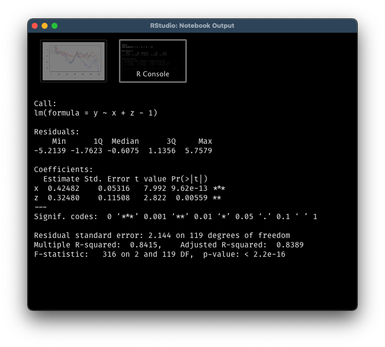
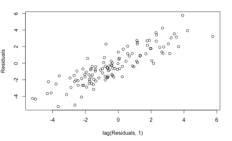
If you are well-versed in regression model, you will notice something wrong immediately by performing residuals analysis. The residuals are highly auto-correlated, a clear violation of OLS assumption.

plot(head(linear_reg$residuals, -1), tail(linear_reg$residuals, -1), xlab = "lag(Residuals, 1)", ylab = "Residuals")
car::durbinWatsonTest(linear_reg)

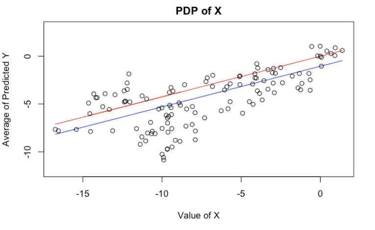
We can, of course, plot PDP’s of $X$ and $Z$. Here, I have plotted the theoretical PDP of $X$ in red, and estimated PDP’s in blue (Exercise: They are somewhat different. Why? Which one better represents the model behavior?). Again, it’s telling us the same wrong story.

plot(x = x[order(x)],
     y = (x[order(x)]*(linear_reg$coefficients[1]) + mean(z)*(linear_reg$coefficients[2])),
     type = "l", col = "blue", ylim = c(-12, 3),
     xlab="Value of X", ylab="Average of Predicted Y", main = "PDP of X")
lines(x, (linear_reg$coefficients[1])*x, col = "red")
points(x, y)

Tree-based algorithms suffer from the same issue

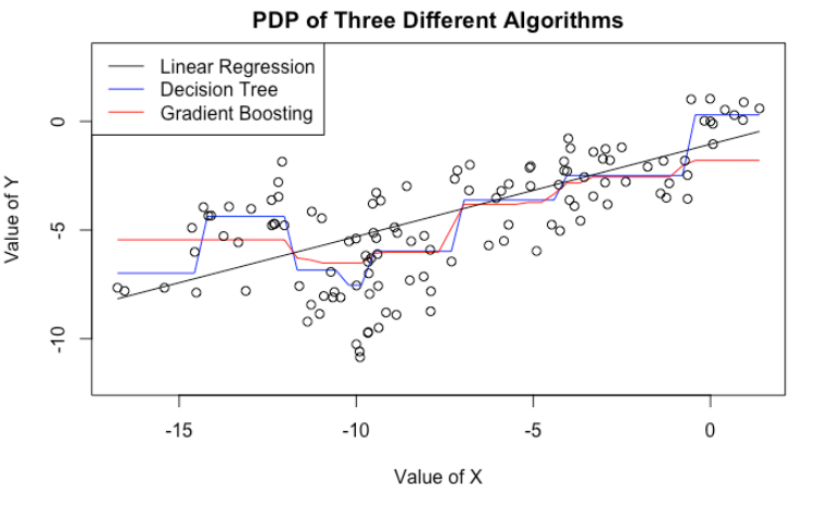
The previous example might be somewhat artificial. After all, I guess very few people would use PDP on linear regressions. However, it gets the point across. Even though tree-based algorithms (e.g. decision tree, gradient boosting, random forest) are more complicated, they still suffer from the same issue.

Here, we fit a decision tree as well as a gradient boosting model to the same data. We then plot their PDP’s on the variable $X$. Even though CART and GBM have more complicated PDP’s (no longer a straight line), they still tell the same story: If we increase $X$, we tend to get a bigger predicted $Y$.

In fact, we are in a worse situation. Because CART/GBM tend to produce more complicated PDP’s, we are more tempted to look for patterns and stories that do not exist. For example, both CART/GBM suggest that when $X$ is near $-10$, we see a dip in $\hat{Y}$. What could be the story behind it? We know there is none, because we know how the data is generated. But in practice, it will be very difficult to tell.

library(gbm)
library(pdp)
library(rpart)

cart_tree <- rpart::rpart(y ~ x + z, method = "anova", control = rpart.control(minsplit = 2))
cart_pdp <- pdp::partial(cart_tree, train = data.frame(x = x, z = z, y = y), pred.var = "x", plot = FALSE)

gbm_model <- gbm::gbm(y ~ x + z + 0,
                      data = data.frame(x = x, z = z, y = y),
                      distribution = "gaussian", n.trees = 50, cv.folds = 10)
gbm_pdp <- pdp::partial(gbm_model, train = data.frame(x = x, z = z, y = y), pred.var = "x", plot = FALSE, n.trees = 45)

plot(x = cart_pdp$x, y = cart_pdp$yhat, col = "blue", type = "l", ylim = c(-12, 3), xlab = "Value of X", ylab = "Value of Y",
     main = "PDP of Three Different Algorithms")
lines(x = gbm_pdp$x[order(gbm_pdp$x)],
      y = gbm_pdp$yhat[order(gbm_pdp$x)], col = "red")
lines(x = x[order(x)],
      y = (x[order(x)]*(linear_reg$coefficients[1]) + mean(z)*(linear_reg$coefficients[2])))
points(x, y)
legend("topleft", legend = c("Linear Regression","Decision Tree","Gradient Boosting"), col = c("black", "blue", "red"), lty=1:1)

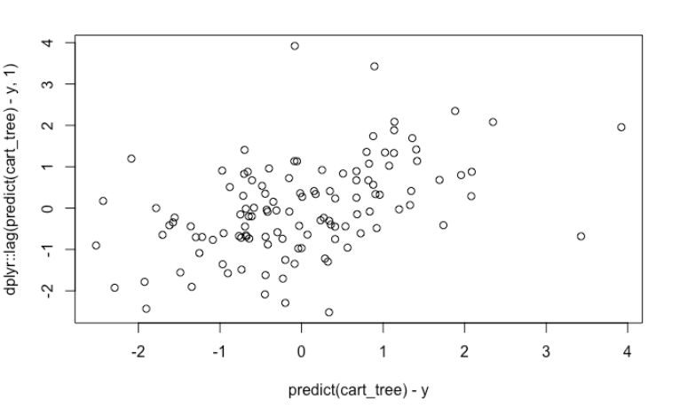
If we have the habit of always doing residual analysis, we can still see some obvious auto-correlation. However, if we forgot to do that, then there is nothing that could hint us the uselessness of our PDP’s.

plot(predict(cart_tree) - y, dplyr::lag(predict(cart_tree) - y, 1))

Start with classical models

In conclusion, when you want to analyze some time series data, it’s probably a good idea to start with some classical models, such as VAR/VARX models. At least for these models, you know clearly what the assumpsion are and how to interpret the model. For example, you can also use impulse response function (IRF) to understand how $Y$ might change over time when you change $X$. On the other hand, tree-based methods are not built with time series in mind. Indeed, none of the popular tree implementations examines residuals and its auto-correlation/stationarity after each split.

References

1. https://scikit-learn.org/stable/modules/partial_dependence.html#mathematical-definition
2. http://statmath.wu.ac.at/~hauser/LVs/FinEtricsQF/FEtrics_Chp4.pdf