Some technical discussions on behaviour of decision tree splitting (cont'd)

Swapping elements to reduce $SS$

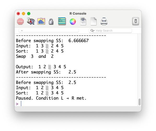
Although we omit the proof, we show how to reduce $SS$ by swapping using a demo. Let’s take $L = \{1,3\}, R = \{2,4,5\}$ as an example.

SS <- function(v) PreciseSums::fsum((v - mean(v))^2)

L_array <- c(1,3)
R_array <- c(2,4,5)

while (TRUE) {
  cat("------------------------------------\n")
  # Make sure L has smaller average
  if (mean(L_array) > mean(R_array)) {
    tp <- L_array
    L_array <- R_array
    R_array <- tp
  }
  
  ss_before_swap <- SS(L_array) + SS(R_array)
  cat("Before swapping SS: ", ss_before_swap, "\n")
  cat("Input: ", L_array, "░", R_array, "\n")
  
  L_array <- sort(L_array)
  R_array <- sort(R_array)
  
  cat("Sort:  ", L_array, "░", R_array, "\n")
  
  # Check if max(L_array) <= min(R_array). If not, swap them
  if (L_array[length(L_array)] > R_array[1]) {
    cat("Swap ",L_array[length(L_array)], " and ", R_array[1],"\n")
    right_most <- L_array[length(L_array)]
    left_most <- R_array[1]
    L_array[length(L_array)] <- left_most
    R_array[1] <- right_most
    
    ss_after_swap <- SS(L_array) + SS(R_array)
    
    cat("\nOutput: ", L_array, "░", R_array, "\n")
    cat("After swapping SS:  ", ss_after_swap, "\n")
  } else {
    cat("Paused. Condition L ⊲ R met.\n")
    break
  }
}

Because there are only 15 partitions for $\{1,2,3,4,5\}$, we can even plot all of them.

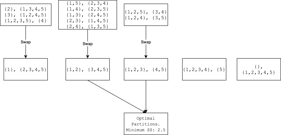
In conclusion, to find the optimal partition, it is best to work with the sorted $\mathbf{y}$. By going through all $n$ possible partitions, we are guaranteed to minimize the impurity $SS(L) + SS(R)$. If $\mathbf{y}$ is not sorted, then there is no guarantee.

Notice that if there are $l$ elements in the optimal left partition, then there are $l!(n-l)!$ possible permutations of $\mathbf{y}$ that guarantees an optimal partition if you do a linear scan. So, if $\mathbf{y}$ is in a random order, then the chance of finding the optimal partition using a linear scan on $\mathbf{y}$ is $\frac{l!(n-l)!}{n!}$. This is extremely small.$^{1}$.

Find $\mathbf{x}$ that is close to $\mathbf{y}$.

Built upon what we have analyzed, we can see why the idea “find the $\mathbf{x}$ strongly correlated with $\mathbf{y}$” could be right or wrong. Intuitively, if $\mathbf{x}$ and $\mathbf{y}$ has exactly the same order, then we will sort $\mathbf{y}$ when we sort $(\mathbf{x}_i, \mathbf{y})$ together using $\mathbf{x}_i$. As we have explained, an ordered $\mathbf{y}$ will guarantee us the optimal partition.

But we have also seen that an unordered $\mathbf{y}$ might give you the minimum $SS$, too. We just need to make sure that after we sort $(\mathbf{x}_i, \mathbf{y})$ together using $\mathbf{x}_i$, one of the $(L, R)$ partition is the same as the optimal one, up to permutation within $L$ and $R$ respectively.

Indeed, the following statements are both wrong.

An incorrect statement: Given features $X_1,\cdots,X_n$ and a response $Y$, a decision tree always chooses the $X_i$ that maximizes its Pearson correlation with $Y$.

Another incorrect statement: Given features $X_1,\cdots,X_n$ and a response $Y$, a decision tree always chooses the $X_i$ that maximizes its Spearman’s correlation with $Y$.

Here are the counterexamples.

# Counterexample to statement 1
Ckmeans.1d.dp::Ckmeans.1d.dp(c(1,2,3,4,5,6), k = 2)

train_df <- data.frame(X1 = c(1,3,4,5,6,7),
                       X2 = c(1,4,5,6,7,8),
                       Y  = c(1,2,3,4,5,6))

stats::cor.test(train_df$X1, train_df$Y, method = 'spearman')$estimate
stats::cor.test(train_df$X2, train_df$Y, method = 'spearman')$estimate

# Counterexample to statement 2
train_df <- data.frame(X1 = c(1,2,6,3,4,5),
                       X2 = c(3,1,2,6,5,4),
                       Y  = c(1,2,3,4,5,6))

In counterexample 2, $\mathbf{x}_1$ has higher Spearman’s correlation with $\mathbf{y}$ than $\mathbf{x}_2$ (0.657 versus 0.6). However, if we use $\mathbf{x}_1$ to sort our $\mathbf{y}$ and look for the best partition, the minimum $SS$ will be $5.5$. On the contrary, if we use $\mathbf{x}_2$, the minimum SS is $4$, which is better.

Going back to the original question

So, going back to the original question,

Is there any smarter way to find the best feature $\mathbf{x}$, without going through all the features? If not, is there any smarter way to understand the whole process at least?

At least for now, the answer is “no”. But it was a fun exercise.

Footnotes:

$^{1}$ We implicitly assume that there is only one optimal partition. This is not the case. For example, $\{1,2,3,4,5\}$ have two different partitions both giving the smallest $SS$, 2.5. Is it possible to have more than 2 partitions such that they all give the smallest $SS$?

I appreciate my friend Tai Yang for taking time to discuss this problem with me.