How useful are PDP's to analyzing time series data?
10 Aug 2021 [statistics decision-tree time-series How useful are PDP’s to analyzing time series data? If you only care about forecast, then there is literally nothing stopping you from doing anything (e.g. “changing the card”). If you mainly care about extracting insights and valid statistical inference, however, they are as useful (or useless) as the coefficients and p-value’s of a linear regression model. A good starting point would be some classical statistical methods (e.g. VAR model) instead of LightGBM.
What is partial dependence plot (PDP)?
Assume the data is generated by some model $Y = f(X_1, \cdots, X_n)$. The partial dependence of $Y$ on $X_i$ is defined as $g(X_i = x) = \mathbb{E}[ f(X_1,\cdots,X_i = x, \cdots,X_n)]$. In other words, it tells you when $X_i = x$, what will predicted $Y$ be in expectation. Note that, in practice, we rarely know the actual DGP. As a result, we use sample average to estimate PDP and almost always get a wiggly curve. For details on PDP, see reference [1].
Here is a very simple example. Assume that $Y = 0.3 X_1 + 0.7 X_2 + \epsilon$, where $X_1, X_2,$ and $\epsilon$ are all normally distributed with mean $2$. What does the PDP of $X_1$ look like? Following the definition, we see that the PD function is just $g(x) = 0.3x + 0.2 \times 2 + 2 = 0.3x + 2.4$. It’s just a straight line.
Here we have our first important takeaway: For linear regression model, PDP and coefficient estimates are “the same thing”. As a result, PDP is reliable if and only if coefficient estimates are reliable.
But OLS coefficient estimates are often not reliable for time series
It is widely known that running OLS on non-stationary time series might give you unreliable results (i.e. spurious regression). For more details, see page 9 of reference [2]. As a result, its PDP’s are not reliable either.
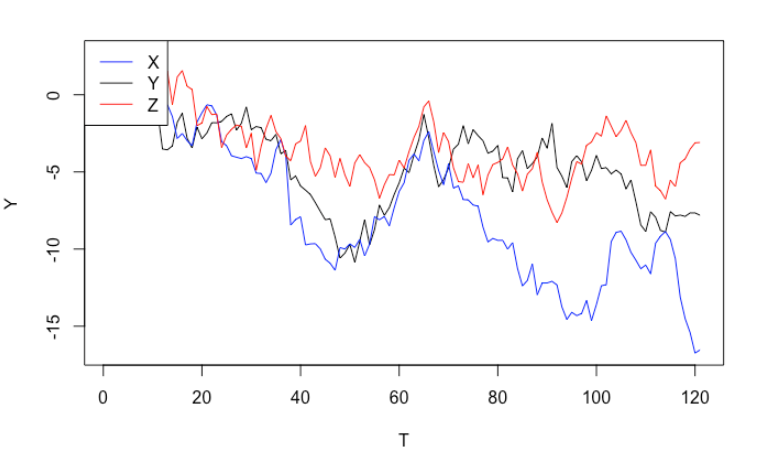
For simplicity, assume we have three time series $X_t, Z_t$ and $Y_t$ that all seem to be “trending downwards”. We want to decide if $X_t$ and/or $Z_t$ are “related to” $Y_t$. Is it possible to figure out by using linear regression? For example, can we rely on coefficient estimate/confidence interval?
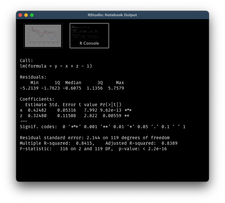
The answer is no. Let’s simulate three independent random walks (note: random walks are non-stationary). From the graph, it seems that all of them are trending downwards, which may trick us to believe that they are related to each other, or we can even use $X_t$ and $Z_t$ to explain $Y_t$. If we run a linear regression formally, it only reconfirms out incorrect conclusion. Even better, the two significant p-values will lead us further down the wrong path.
set.seed(24)

n <- 12*10
x <- c(0, cumsum(rnorm(n)))
y <- c(0, cumsum(rnorm(n)))
z <- c(0, cumsum(rnorm(n)))

ylab_min <- min(c(x, y, z))
ylab_max <- max(c(x, y, z))
plot(y, type = "l", ylim = c(ylab_min, ylab_max), xlab = "T", ylab = "Y")
lines(x, col = "blue")
lines(z, col = "red")
legend("topleft", legend = c("X","Y","Z"), col = c("blue", "black", "red"), lty=1:1)

linear_reg <- lm(y ~ x + z - 1)
summary(linear_reg)
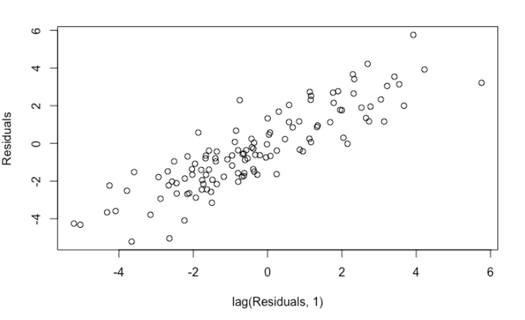
If you are well-versed in regression model, you will notice something wrong immediately by performing residuals analysis. The residuals are highly auto-correlated, a clear violation of OLS assumption.
plot(head(linear_reg$residuals, -1), tail(linear_reg$residuals, -1), xlab = "lag(Residuals, 1)", ylab = "Residuals")
car::durbinWatsonTest(linear_reg)
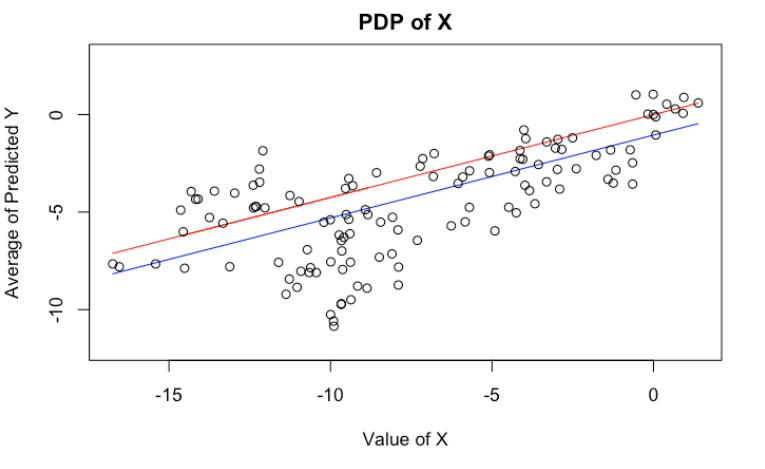
We can, of course, plot PDP’s of $X$ and $Z$. Here, I have plotted the theoretical PDP of $X$ in red, and estimated PDP’s in blue (Exercise: They are somewhat different. Why? Which one better represents the model behavior?). Again, it’s telling us the same wrong story.
plot(x = x[order(x)],
     y = (x[order(x)]*(linear_reg$coefficients[1]) + mean(z)*(linear_reg$coefficients[2])),
     type = "l", col = "blue", ylim = c(-12, 3),
     xlab="Value of X", ylab="Average of Predicted Y", main = "PDP of X")
lines(x, (linear_reg$coefficients[1])*x, col = "red")
points(x, y)
Tree-based algorithms suffer from the same issue
The previous example might be somewhat artificial. After all, I guess very few people would use PDP on linear regressions. However, it gets the point across. Even though tree-based algorithms (e.g. decision tree, gradient boosting, random forest) are more complicated, they still suffer from the same issue.
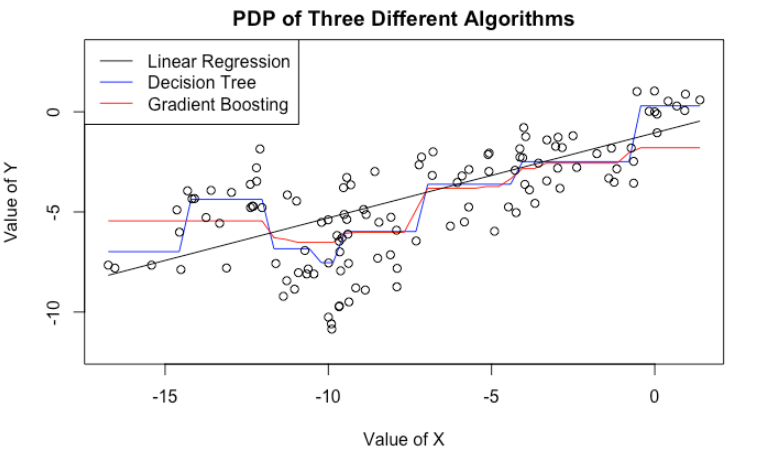
Here, we fit a decision tree as well as a gradient boosting model to the same data. We then plot their PDP’s on the variable $X$. Even though CART and GBM have more complicated PDP’s (no longer a straight line), they still tell the same story: If we increase $X$, we tend to get a bigger predicted $Y$.
In fact, we are in a worse situation. Because CART/GBM tend to produce more complicated PDP’s, we are more tempted to look for patterns and stories that do not exist. For example, both CART/GBM suggest that when $X$ is near $-10$, we see a dip in $\hat{Y}$. What could be the story behind it? We know there is none, because we know how the data is generated. But in practice, it will be very difficult to tell.
library(gbm)
library(pdp)
library(rpart)

cart_tree <- rpart::rpart(y ~ x + z, method = "anova", control = rpart.control(minsplit = 2))
cart_pdp <- pdp::partial(cart_tree, train = data.frame(x = x, z = z, y = y), pred.var = "x", plot = FALSE)

gbm_model <- gbm::gbm(y ~ x + z + 0,
                      data = data.frame(x = x, z = z, y = y),
                      distribution = "gaussian", n.trees = 50, cv.folds = 10)
gbm_pdp <- pdp::partial(gbm_model, train = data.frame(x = x, z = z, y = y), pred.var = "x", plot = FALSE, n.trees = 45)

plot(x = cart_pdp$x, y = cart_pdp$yhat, col = "blue", type = "l", ylim = c(-12, 3), xlab = "Value of X", ylab = "Value of Y",
     main = "PDP of Three Different Algorithms")
lines(x = gbm_pdp$x[order(gbm_pdp$x)],
      y = gbm_pdp$yhat[order(gbm_pdp$x)], col = "red")
lines(x = x[order(x)],
      y = (x[order(x)]*(linear_reg$coefficients[1]) + mean(z)*(linear_reg$coefficients[2])))
points(x, y)
legend("topleft", legend = c("Linear Regression","Decision Tree","Gradient Boosting"), col = c("black", "blue", "red"), lty=1:1)
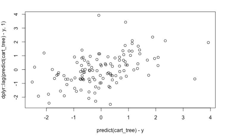
If we have the habit of always doing residual analysis, we can still see some obvious auto-correlation. However, if we forgot to do that, then there is nothing that could hint us the uselessness of our PDP’s.
plot(predict(cart_tree) - y, dplyr::lag(predict(cart_tree) - y, 1))
Start with classical models
In conclusion, when you want to analyze some time series data, it’s probably a good idea to start with some classical models, such as VAR/VARX models. At least for these models, you know clearly what the assumpsion are and how to interpret the model. For example, you can also use impulse response function (IRF) to understand how $Y$ might change over time when you change $X$. On the other hand, tree-based methods are not built with time series in mind. Indeed, none of the popular tree implementations examines residuals and its auto-correlation/stationarity after each split.
References